-
Notifications
You must be signed in to change notification settings - Fork 1
MetaFX tutorial
Here is presented a MetaFX tutorial based on simulated bacterial metagenomes. It provides a step-by-step analysis of metagenomics data from raw reads to samples categories prediction.
- Input data
- Feature extraction from train data
- Train data analysis
- Test data processing
- Test data prediction
It is highly recommended to run this tutorial on computational cluster due to high resource requirements.
Disk storage: 30Gb of free disk space is required. ~12Gb for input data and ~16Gb for intermediate computational steps.
RAM: 8Gb should be enough.
Threads: with 6 threads this tutorial took 1 hour to run. More threads will speed up the computations, especially k-mers extraction step.
We will use in-silico metagenomic data generated with InSilicoSeq. For comparative analysis at least two groups (categories) of metagenomes are required – A and B. In each group there are two types of samples – train and test. Train data will be used for feature extraction and classification model training. Test data is required to validate extracted features and check the accuracy of predictive model.
There are 40 samples in total. Each sample contains 10 random bacteria from a predefined pool of 20 bacteria. Additionally, all samples contain E.coli strain, different between A and B groups. These strains are quite similar, with mash distance D=0.022 (i.e. Average Nucleotide Identity ANI≈0.978). Dataset overview is presented in the table below.
| group A | group B | ||
| train | test | train | test |
| 10 samples | 10 samples | 10 samples | 10 samples |
| 10 random bacteria from 20 | |||
| E.Coli str. K-12 | E.coli O157:H7 str. Sakai | ||
Raw data can be download by [this link](/metafx_tutorial/data.zip). Alternatively, you can run the following command:
wget <TODO>/metafx_tutorial/data.zipFurther we need to extract data and delete the archive:
unzip data.zip
rm data.zip
data/ directory contains several files and folders:
-
data/reads/contains 80 files with paired-end reads for 40 samples. -
data/species_distribution.tsvcontains the relative abundance of bacterial species in samples. -
data/train_dataset.txtcontains path to train samples and their categories. -
data/test_labels.txtcontains information about test samples and their categories.
We can examine bacterial content with:
cat data/species_distribution.tsv
Now we are ready to start data analysis. We will use train data to extract features, which are different between A and B groups.
MetaFX can take as input raw sequencing reads data, but it can also be provided with pre-computed k-mers for speed up. Splitting reads into k-mers can take some time, but this can be done once and k-mers can be stored on hard drive. This can be especially useful, if you plan to run several MetaFX modules for feature extraction, or want to try the same module with different parameters.
Thus, we start with splitting input reads into k-mers.
metafx extract_kmers -t 6 -m 8G -w wd_kmers_train -k 31 -i data/reads/A_train_*.fastq.gz data/reads/B_train_*.fastq.gzAs a result wd_kmers_train/ directory will be created, which stores kmers/ folder with binary k-mers files for each sample. It can be provided to other MetaFX modules through --kmers-dir parameter.
This step will take approximately 15 minutes with 6 threads, but can be further speed up, if you have more cores. Alternatively, you can download the resulting folder by [this link](/metafx_tutorial/wd_kmers_train.zip) or by
wget <TODO>/metafx_tutorial/wd_kmers_train.zipMetaFX supports several algorithms for feature extraction based on samples categories. We will use unique module to extract features based on k-mers, unique for each group (A and B in our case).
As input we should provide information about where to find input samples and which categories they belong to. This information should be in one tab-separated file and we have it in data/train_dataset.txt file.
Also, we will pass wd_kmers_train/kmers directory with pre-computed k-mers into --kmers-dir parameter.
Thus, we run command
metafx unique -t 6 -m 8G -w wd_unique -k 31 -i data/train_dataset.txt --kmers-dir wd_kmers_train/kmersAs a result, we obtain wd_unique directory with extracted features. This step will take approximately 20 minutes with 6 threads. Alternatively, you can download the resulting folder by [this link](/metafx_tutorial/wd_unique.zip) or by
wget <TODO>/metafx_tutorial/wd_unique.zipDirectory contains:
-
wd_unique/categories_samples.tsv– file with categories present in input data and corresponding samples. -
wd_unique/samples_categories.tsv– file with input samples and their respective categories. -
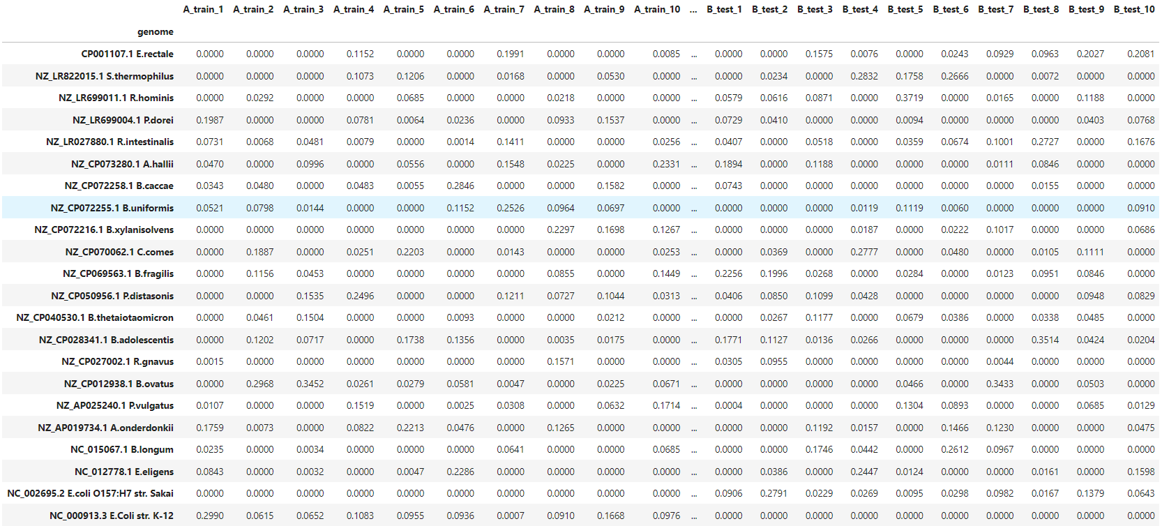
wd_unique/feature_table.tsv– table with feature values for all samples.
We will look closer to feature_table.tsv file. Firstly, let's check its structure.
$ head -n 5 wd_unique/feature_table.tsv
	B_train_1	B_train_4	A_train_9	A_train_7	A_train_10	A_train_2	B_train_6	B_train_5	A_train_4	A_train_5	A_train_6	B_train_2	A_train_8	B_train_8	A_train_3	B_train_9	B_train_3	B_train_7	B_train_10	A_train_1
A_0	0.5704682116073239	0.5539659482467401	0.9949834470643876	0.0021197892034322007	0.9942064725356394	0.9795875278697386	0.5704682116073239	0.5273714613877439	0.9943669346665766	0.9944513884197014	0.99342105263157910.5678754813863928	0.9943500439159516	0.5703499763529492	0.9797142084994256	0.3066853590973583	0.5687622457942031	0.5704682116073239	0.5694040943179515	0.9976437402878184
A_1	0.5181385649740535	0.5008089548303591	0.9955417600460206	0.004841744466149735	0.9932527174890042	0.9747126712287724	0.5180426888460109	0.4746347718747378	0.9944272000575256	0.994067664577366	0.992797305880802	0.5147709159765583	0.9926534916887382	0.517970781749979	0.9801536414951882	0.2996248846490335	0.5175153701417768	0.5180426888460109	0.5176112462698194	0.9970278400306803
A_2	0.21169835256201466	0.2073268990108515	0.9957485471345552	0.0028971594123394988	0.9945142543671678	0.9816227521300122	0.21169835256201466	0.19342396242264245	0.9947028268732964	0.9948228275590146	0.99511425779575880.21102977731301326	0.9946513980079886	0.21147549414568084	0.9865084943342534	0.13836079063308934	0.21169835256201466	0.21169835256201466	0.21145835119057824	0.998405705175458
A_3	0.6681529053238705	0.653958644386722	0.9955617368539464	0.0019839240791115287	0.9942936616693596	0.9758247601906204	0.6681119996727548	0.6109258994130039	0.994927699261653	0.993680076902624	0.99212566216022760.6658212832102754	0.9945595484016116	0.6675597733826928	0.9842104186693392	0.39142617552614895	0.6662098868958747	0.6681119996727548	0.6671098112204201	0.9993659624077066
First row contains samples names. First column contains extracted features' names in format <Category of feature>_<number of feature>. Features are represented as floating-point numerical values.
$ wc -l wd_unique/feature_table.tsv
3372 wd_unique/feature_table.tsv
Secondly, let's get the number of features. Totally, 3371 features were extracted.
At this step we can work with extracted features. We will visualise data based on features and train a predictive model.
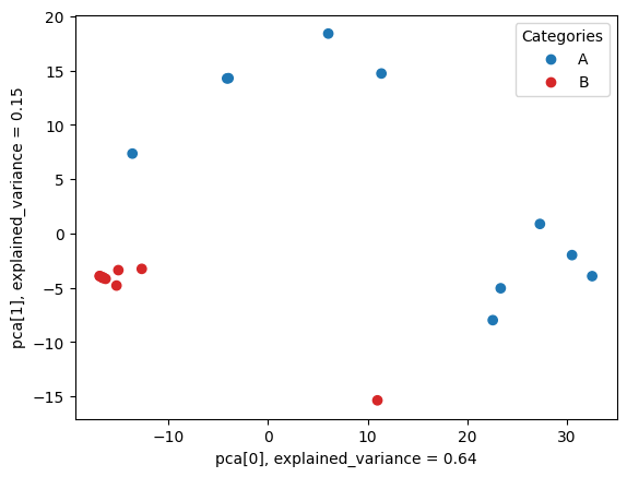
We will use dimensionality reduction to visualise the clusters in train data and check the utility of extracted features. For Principal Component Analysis (PCA) we need to provide feature table and samples' labels.
metafx pca -w wd_pca -f wd_unique/feature_table.tsv -i wd_unique/samples_categories.tsvAs a result, we obtain wd_pca/pca.png image, which clearly shows two separate clusters of A and B samples.

Next we will use extracted features to train classification machine learning model capable of predicting categories for test samples.
metafx fit -w wd_fit -f wd_unique/feature_table.tsv -i wd_unique/samples_categories.tsvAs a result, we obtain wd_fit/rf_model.joblib file with pre-trained model for category prediction. We will use this model in the following steps to predict categories of test samples.
And now we will work with test data. We will count numerical feature values based on features, constructed from train samples. Also, we will check the validity of extracted features based on their ability to predict categories for test samples.
First of all, we need to extract k-mers from test samples' reads, as we did for train data.
metafx extract_kmers -t 6 -m 8G -w wd_kmers_test -k 31 -i data/reads/A_test_*.fastq.gz data/reads/B_test_*.fastq.gzAs a result wd_kmers_test/ directory will be created, which stores kmers/ folder with binary k-mers files for each sample. It can be provided to other MetaFX modules through --kmers-dir parameter.
This step will take approximately 15 minutes with 6 threads, but can be further speed up, if you have more cores. Alternatively, you can download the resulting folder by [this link](/metafx_tutorial/wd_kmers_test.zip) or by
wget <TODO>/metafx_tutorial/wd_kmers_test.zipNext, we need to obtain feature values for test samples based on previously extracted features. We use directory with features wd_unique/ and k-mers for test samples wd_kmers_test/kmers/.
metafx calc_features -t 6 -m 8G -w wd_calc_features -k 31 --kmers-dir wd_kmers_test/kmers -d wd_unique/As a result, we obtain wd_calc_features/feature_table.tsv file with extracted features for test samples. This step will take approximately 1 minute with 6 threads. Alternatively, you can download the resulting folder by [this link](/metafx_tutorial/wd_calc_features.zip) or by
wget <TODO>/metafx_tutorial/wd_calc_features.zipFinally, we are ready to perform an analysis of test samples. We will use MetaFX predict module to get hidden test samples categories based on extracted features and pre-trained model.
metafx predict -w wd_predict -f wd_calc_features/feature_table.tsv --model wd_fit/rf_model.joblib -i data/test_labels.txtAs a result, we obtain wd_predict/predictions.tsv file with predicted category label for each test sample.
$ cat wd_predict/predictions.tsv
A_test_5	A
B_test_7	B
A_test_7	A
B_test_9	B
A_test_1	A
A_test_4	A
B_test_3	B
A_test_10	A
A_test_8	A
B_test_8	B
B_test_10	B
B_test_6	B
B_test_2	B
A_test_2	A
A_test_9	A
B_test_4	B
A_test_6	A
B_test_1	B
A_test_3	A
B_test_5	A
As we can see, only one samples (B_test_5) was misclassified.
Since we provided -i data/test_labels.txt parameter with hidden labels, we obtained in the log output the accuracy of our model. In real data with absent knowledge about correct labels, this parameter can be omitted.
Predictions accuracy compared with given labels:
              precision    recall  f1-score   support

           A       0.91      1.00      0.95        10
           B       1.00      0.90      0.95        10

    accuracy                           0.95        20
   macro avg       0.95      0.95      0.95        20
weighted avg       0.95      0.95      0.95        20