<<<<<<< HEAD
This repo contains some basic techniques for processing Digital Signals.
- Analog signals are present all around us, may it be temperature, heart rate or sound;
- These signals need to be converted to digital form so that our computers can process and analyse the signals easily;


- So, I will include some signal processing techniques that I do in my lab along with some additional information to get you started;
- The motivation behind this is after getting yourself acquainted with the methods you can explore more in the world of sensors, IoT, data processing and much more;
- Arduino Due(Arduino Uno may not support the processing strength required);

Arduino Due has 96 kilo bytes SRAM and 512 kilo bytes flash memory.
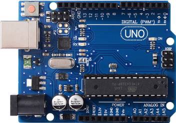
Arduino Uno has 2 kilo bytes SRAM and 32 kilo bytes flash memory
- MATLAB(Octave or Python may also serve as an alternative to visualize plots);
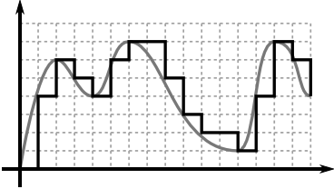
- Filter is a system that either allows or rejects specific frequency components in the input to produce an output.
- There are many types of filters:
- Low Pass Filter
- High Pass Filter
- All Pass Filter
- Band Pass Filter
- Band Stop Filter
- Notch Filter
- The three filters in focus here are:
- Moving average filter-A low pass filter
- First order difference filter-A high pass filter
- Three point central difference filter-A band pass filter
- Moving Average Filter:

Input/Output relation

Converting to Z-Transform
![]()
Transfer function equation
- First order difference filter:

Input/Output relation
![]()
Transfer function equation
- Three point central difference filter:

Input/Output relation
![]()
Transfer function equation
- Moving Average Filter:

Pole-Zero plot for L=2

Magnitude Response

Phase Response

Pole-Zero plot for L=8

Magnitude Response

Phase Response

Pole-Zero plot for L=100

Magnitude Response

Phase Response
- First order difference filter:

Pole-Zero plot

Magnitude Response

Phase Response
- Three point central difference filter:

Pole-Zero plot

Magnitude Response

Phase Response
- The given data set is that of ppg signal of 1000 sample points and sampled at 100Hz;
- Moving average filter results:

L=2; Blue-PPG signal, Red-Moving averaged ppg signal

L=8; Blue-PPG signal, Red-Moving averaged ppg signal

L=100; Blue-PPG signal, Red-Moving averaged ppg signal
- High Pass Filters:

Blue-PPG signal, Red-Moving averaged ppg signal, Green- First Order Difference

Blue-PPG signal, Red-Moving averaged ppg signal, Green- Three Point Difference
- Removing Baseline Drift:

Blue-PPG signal, Red-Noide(first order difference), Green- PPG Signal without noise, Yellow- Moving averaged ppg signal, Purple- Baseline component, Indigo- PPG signal without baseline component
- Moving average on difference operator:

Blue-PPG signal, Red-Noide(first order difference), Green- Moving averaged first order difference
This lab is based on applying autocorrelation function to PPG signal and Speech signal.
- Autocorrelation is defined as the correlation of signal with a delayed copy of itself;

Autocorrelation equation for continuous time domain
-
Properties of autocorrelation signal:
- Autocorrelation function is a function of delay;
- It is an even signal;
- It has maximum at zero delay;
- It ranges from -1 to 1 and slowly dies out to 0 when delay is same as the length of the signal;
-
Applications of autocorrelation include:
- Detection of periodicity in a signal obscured by noise;
- Detection of missing fundamental frequency in signal;
- Removal of white noise;
-
Detection of periodicity in signal:
- From autocorrelation function we need to find the first zero crossing location;
- From the first zero crossing location we need to find the location of the first maximum;
- Doing so tells us after how much delay(shifting) there will be a strong similarity(hence periodicity);
- Period(or Pitch period) is calculated as (True location of second maximum)/(Sampling frequency);
- PPG stands for Photoplethysmogram, where 'plethys' means measuring volume of an organ;
- Hence, PPG tries to capture heart rate information by measuring how much light is absorbed at the tips of our fingers;
- The heart rate obtained is called pulse period;
- Pulse period is defined as (60/pitch period) where pitch period is determined by autocorrelation technique;
- It is the resting pulse period and is measured in beats per minute(BPM);
- Dataset of PPG signal contains 2000 samples sampled at 100Hz

Blue-PPG signal;Red-Moving Averaged PPG Signal;Green- Autocorrelation signal

Obtained results for pulse period
- Speech signal is produced by our voice box;
- For males, it is in range 65 to 260 Hz(approximately);
- For females, it is in range 100 to 525 Hz(approximately);
- Pitch frequency can be calculated using autocorrelation as mentioned above;
- Pitch frequency is found as (1/Pitch period);

Blue-PPG signal;Red-Moving Averaged PPG Signal;Green- Autocorrelation signal

Obtained results for pitch frequency
- Real world signals are analog signals that is continuous in time, hence infinite values;
- Since, computer cannot handle infinite values, it needs to be sampled in time domain;
- To get frequency spectrum of sampled signal, we perform Discrete Time Fourier Transform(DTFT);
- But the spectrum of DTFT is continuous and needs to be sampled;
- So, sampling in frequency domain leads to Discrete Fourier Transform(DFT);

Discrete time fourier transform formula

Discrete fourier transform formula
- First, one moving averages the signal to smoothen it and remove high frequency noises;
- Then, one takes the DFT of the signal and finds the k index for which magnitude response is maximum;
- The first peak is taken in magnitude response;
- The corresponding frequency for a k index is (kindex.sampling frequency)/(length of signal);
- The pulse rate is obtained as (60 . pitch frequency[as computed above]);

DFT Spectrum showing periodicity(repeatitions)

DFT spectrum without moving average filter

DFT spectrum with moving average filter
ARDUINO Implementation Code
const int L=75;
const int N=75;
float pi=3.141593522;
float sig[75]={-87.1730763754109}; //75 samples
float Fs=25;//25 Hz, sampling frequency
float* movavg=new float[75]; //moving average array
int window=20; //moving average window
float* dftReal=new float[75]; //array to store real values of dft of signal
float* dftImag=new float[75]; //array to store imaginary values of dft of signal
float** dftmatrixRealPart=new float*[75]; //array to store real values of dft MATRIX of signal
float** dftmatrixImagPart=new float*[75]; //array to store real values of dft MATRIX of signal
float maxm=-1000;
int kindex=0;


//Frequency is kFs/L;
void setup() {
    Serial.begin(9600);
    for(int i=0;i<75;i++)
    {
     dftmatrixRealPart[i]=new float[75];
     dftmatrixImagPart[i]=new float[75];
      }//2D Array initialization

    for(int n=0;n<L;n++)
    {
      dftmatrixRealPart[0][n]=1;dftmatrixRealPart[n][0]=1;//This block assumes N==L so loop is equal for column and row
      dftmatrixImagPart[0][n]=0;dftmatrixImagPart[n][0]=0;
      }//Inititalizing all values of 1st row and 1st column of real dft matrix to 1 and of imaginary dft matrix to 0

    for(int k=1;k<N-1;k++)
    {
      for(int n=k;n<L;n++)
      {
        dftmatrixRealPart[k][n]=cos((2*pi*k*n)/N);
        dftmatrixImagPart[k][n]=sin((2*pi*k*n)/N)*(-1);
        if(n!=k)
        {
         dftmatrixRealPart[n][k]=dftmatrixRealPart[k][n];
         dftmatrixImagPart[n][k]=dftmatrixImagPart[k][n];
          }
        }
      } //Finding DFT Matrix

     doMovingAverage(sig,movavg,10,75); //doing moving average which is available in helper functions file

     for(int k=0;k<N;k++)
     {
      float sumReal=0,sumImag=0;
      for(int n=0;n<L;n++)
      {
        sumReal+=(dftmatrixRealPart[k][n]*movavg[n]);
        sumImag+=(dftmatrixImagPart[k][n]*movavg[n]);
        }
        dftReal[k]=sumReal;
        dftImag[k]=sumImag;
      }// Multiplying dft matrix with cleaned signal

      for(int k=0;k<(N-1);k++)
      {
        float xy=sqrt((dftReal[k]*dftReal[k])+(dftImag[k]*dftImag[k]));
        if(xy>maxm&&(k<N/2))
        {
          maxm=xy;
          kindex=k;
          }
        } //Finding 1st value of k index for maximum magnitude
        Serial.print("Frequency for maximum magnitude spectrum is ");Serial.print((kindex*Fs)/N);Serial.println(" Hz");
        Serial.print("Pulse period is ");Serial.print(60*(kindex*Fs)/N);Serial.println(" BPM");

}

void loop() {
  for(int k=0;k<(N-1);k++)
  {
    float xy=sqrt((dftReal[k]*dftReal[k])+(dftImag[k]*dftImag[k])); //Printing Spectrum
    Serial.print(xy);
        Serial.println(',');
    }
}
MATLAB Code
y=load('exp4.mat'); %Loading data
x3=y.x3;
x3=x3';
[r,c]=size(x3); % x3 is signal and r is length of signal

%moving average
mov=zeros(r,1);
l=7;
for k=1:r-l
    sum=0.0;
    for z=k:k+l
        sum=sum+x3(z);
    end
    mov(k)=sum/l;
end %Performed moving average
figure(1);
subplot(1,2,1);

% Constructing DFT Matrix
dftmatrix=ones(r,r);
for k=2:r
    for z=k:r
        cvar=exp(-(2*pi*1j*(k-1)*(z-1))/r);
        dftmatrix(k,z)=cvar;
        if(k~=z)
            dftmatrix(z,k)=dftmatrix(k,z);
        end
    end
end

%%DFT multiplication
fs=25;%25Hz sampling frequency;

xkwithoutMA=dftmatrix*x3; %Multiplying signal with dft matrix
xkwithoutMA=abs(xkwithoutMA); %Taking magnitude values
xk=dftmatrix*mov;
xk=abs(xk);
[~,kindex]=max(xk(1:r/2)); %Finding 1st maximum value's location
kindex=kindex-1;
pitchfreq=(kindex*fs)/r; %Calculating pitch frequency
display("Pitch frequency is with Moving Average of window "+l+" is "+60*pitchfreq+" BPM");
[~,kindex]=max(xkwithoutMA(1:r/2));
kindex=kindex-1;
pitchfreq=(kindex*fs)/r;
display("Pitch frequency is without Moving Average is "+60*pitchfreq+" BPM");
Signal Waveform

DFT in MATLAB

Pulse rate found in MATLAB

Pulse rate found with Autocorrelation function

Pulse rate found with DFT method
- Error=(80-71.43)/71.43=0.1199=11.99%
- In last lab, using DFT we found the pulse rate to be 80 beats per minute;
- Here we use ArduinoFFT library to get the pulse rate and verify the results;
- FFT does the work in O(NlogN) while DFT does it in O(N^2)
- FFT can be implemented by Decimation in Frequency/Time(DIF/DIT) techniques;
#include "arduinoFFT.h"

arduinoFFT FFT = arduinoFFT(); /* Create FFT object */
/*
These values can be changed in order to evaluate the functions
*/
const uint16_t samples = 128; //This value MUST ALWAYS be a power of 2
const double samplingFrequency = 25;
/*
These are the input and output vectors
Input vectors receive computed results from FFT
*/
double vReal[samples]={-87.173076375410917...data};
double vImag[samples]={0};
double maxim=-10000.0;int kindex=0;
int window=10;double sum=0;
double vRealMA[samples];

void setup()
{
  Serial.begin(9600);
  for(int i=75;i<128;i++)
    vReal[i]=0;

    //MOVING AVERAGE
  for(int i=(samples-window+1);i<samples;i++)
  vRealMA[i]=0;
  for(int i=0;i<(samples-window+1);i++)
 {
  float sum=0;
  for(int j=i;j<window+i;j++)
  {
   sum+=vReal[j];
   }
   vRealMA[i]=sum/window;
  }

  FFT.Windowing(vRealMA, samples, FFT_WIN_TYP_HAMMING, FFT_FORWARD);  /* Weigh data */
  FFT.Compute(vRealMA, vImag, samples, FFT_FORWARD); /* Compute FFT */
  for(int i=0;i<samples;i++)
  {
    double temp=sqrt(vRealMA[i]*vRealMA[i]+vImag[i]+vImag[i]);
    if((temp>maxim)&&(i<samples/2))
    {
      maxim=temp;kindex=i;
      }
    Serial.print(temp);
    Serial.println(',');
  }
  Serial.print("Pulse rate using FFT Library and with moving average window ");Serial.print(window);Serial.print(" is: ");Serial.print((60*kindex*samplingFrequency)/samples);Serial.println(" BPM");
}
Code to implement FFT library

Spectrum obtained by FFT


Pulse rate results obtained by FFT
- Raw ppg data contains respiratory information too;
- While ppg frequency lies between 0.5 to 5 Hz, respiratory frequency lies between 0.05 to 0.5 Hz;
- Hence, FFT can be used to zero out non respiratory components;
y=load('ppgwithRespiration_25hz_30seconds.mat');
x=y.xppg;
x=x';
[l,~]=size(x);
myfft=fft(x,l);
figure(1);
subplot(1,2,1);
plot(x);axis tight;grid on;title('Input Signal');xlabel('Time');ylabel('Amplitude');
subplot(1,2,2);
plot(abs(myfft));axis tight;grid on;title('Frequency Spectrum');xlabel('Frequency');ylabel('Magnitude');

%Getting respiratory part only
myfft(1)=0;
myfft(17:l,:)=0; %Setting non respiratory components to zero
xapp=ifft(myfft,l);
[~,loc]=max(myfft);
display("Respiratory rate in Breaths per minute: ");display((loc-1)*25*60/l);
figure(2);
subplot(1,2,1);
plot(abs(xapp));axis tight;grid on;title('Respiratory Signal only');xlabel('Time');ylabel('Amplitude');
subplot(1,2,2);
plot(abs(myfft));axis tight;grid on;title('Frequency Spectrum');xlabel('Frequency');ylabel('Magnitude');
Input Signal and Spectrum

Obtained respiratory signal

Respiration rate in Matlab/Octave
#include "arduinoFFT.h"

arduinoFFT FFT = arduinoFFT(); /* Create FFT object */
/*
These values can be changed in order to evaluate the functions
*/
const uint16_t samp2=750;
const uint16_t samples = 1024; //This value MUST ALWAYS be a power of 2
const double samplingFrequency = 300;
/*
These are the input and output vectors
Input vectors receive computed results from FFT
*/
double vRealAll[samp2]={-293.993316,..data};
double vReal[samples];
double vRealMA[samples];
double sig[samples];
double vImag[samples]={0};
int window=1;
double maxm=-1000;int kindex=0;

void setup()
{
  Serial.begin(9600);
    doMovingAverage(vReal,vRealMA,samples,window);

  FFT.Compute(vRealMA, vImag, samples, FFT_FORWARD); /* Compute FFT */
  double* myfft=new double[samples];
  for(int i=0;i<samples;i++)
  {
    myfft[i]=magn(i);
    }

   window=100;
  doMovingAverage(myfft,myfft,samples,window);
  //For getting correct rate it is important to moving average the signal in frequency domain also
  for(int i=0;i<16;i++)
  {
    Serial.print(myfft[i]);
    Serial.println(',');
    }
  for(int k=0;k<samples;k++)
  {
    if(!(k>=1&&k<=15))
    {
      vRealMA[k]=0;vImag[k]=0;
      }
      else
      {
        if(myfft[k]>maxm)
        {
          maxm=myfft[k];kindex=k;
          }
        }
    }
    Serial.print("Respiratory rate is: ");Serial.print(60*(kindex*samplingFrequency)/samples);Serial.println(" breaths per minute");
    FFT.Compute(vRealMA, vImag, samples,FFT_REVERSE); /* Compute Inverse FFT */
}
Extracted respiratory signal

PPG Signal only(Respiratory components removed)

Respiration rate in arduino
Lab 06 onwards documentation is present inside respective folders; Thank you :)
a75e612079e71da393283e09d2d20d23981aa151