Build a Traffic Sign Recognition Project
The goals / steps of this project are the following:
- Load the data set (see below for links to the project data set)
- Explore, summarize and visualize the data set
- Design, train and test a model architecture
- Use the model to make predictions on new images
- Analyze the softmax probabilities of the new images
- Summarize the results with a written report
1. Provide a basic summary of the data set. In the code, the analysis should be done using python, numpy and/or pandas methods rather than hardcoding results manually.
I used the numpy library to calculate summary statistics of the traffic signs data set:
- The size of training set is 34799
- The size of the validation set is 4410
- The size of test set is 12630
- The shape of a traffic sign image is 32x32x3
- The number of unique classes/labels in the data set is 43
Here is an exploratory visualization of the data set. It is a bar chart showing how the training samples are distributed among each traffic sign class.

As you can see the number of training samples of each class varies widely. (I have explained below the steps I have taken to make it more balanced among different classes at preprocessing step.)
1. Describe how you preprocessed the image data. What techniques were chosen and why did you choose these techniques? Consider including images showing the output of each preprocessing technique. Pre-processing refers to techniques such as converting to grayscale, normalization, etc. (OPTIONAL: As described in the "Stand Out Suggestions" part of the rubric, if you generated additional data for training, describe why you decided to generate additional data, how you generated the data, and provide example images of the additional data. Then describe the characteristics of the augmented training set like number of images in the set, number of images for each class, etc.)
As a preprocessing step, I normalized the image data to range of [0,1] using min-max scaling because having large pixel values in the range of [0,255] could cause the network to get saturated and making hard to train the network.
I did not used any other preprocessing like grayscalling or histogram normalization etc. Instead as proposed in "Systematic evaluation of CNN advances on the ImageNet", I used a mini network at the beginning of my model to learn a transformation via convolution. While original paper suggests using 1x1 convolutions, I used 3x3 and 1x1 convolutions respectively at this step which gave better results.
I decided to generate additional data because it helps to prevent model from over fitting on training set since samples were not equally distributed between each classes in the original training set.
To add more data to the data set, I used the following techniques because they would generate as much as legitimate samples without introducing unrealistic image effects to the training samples.
First I used flipping of existing samples of symmetrical signs wherever possible. For this I used the flipping method available at, https://navoshta.com/traffic-signs-classification/#flipping
Then I balanced the data between classes by cloning existing samples so that there are at least 2000 samples per each class. At each iteration of training a randomly selected portion of these were perturbed using random translations, rotations and perspective transformations. In this step I also used border reflect method to prevent introducing high contrast unwanted features and keep the border areas consistent with original images. The basic idea of this approach is to create "infinite" augmented training data set by generating new data during the training epoch. When training data is always changing, the network will be less prone to over fitting. However at the same time it is necessary to make sure that the data change is not too big so that it won't cause "jumps" in the training loss.
Here is an example of an original image and an augmented image:

The difference between the sample counts in original data set and the augmented data set is the following.
- The size of extended training set is 112134
- Minimum number of samples per class in original data set is 180
- Maximum number of samples per class in original data set is 2010
- Minimum number of samples per class in extended data set is 2010
- Maximum number of samples per class in extended data set is 7560
Note that due to few classes that had high number of symmetrical traffic signs there were few outliers that got high number of samples than average of 2000 samples after this operation.
2. Describe what your final model architecture looks like including model type, layers, layer sizes, connectivity, etc.) Consider including a diagram and/or table describing the final model.
My final model consisted of the following layers:
| Layer | Description |
|---|---|
| Preprocessing Mini-Net | |
| Input | 32x32x3 RGB image |
| Convolution 3x3 | 1x1 stride, same padding, outputs 32x32x10 |
| Batch normalization | |
| VLReLU (alpha=0.25) | |
| Convolution 1x1 | 1x1 stride, same padding, outputs 32x32x3 |
| Batch normalization | |
| VLReLU (alpha=0.25) | |
| Densenet Model | |
| Convolution 5x5 | 1x1 stride, same padding, outputs 32x32x32 |
| Dense block | growth rate:24, 4 layers, outputs 32x32x128 |
| Batch normalization | |
| ReLU | |
| Convolution 1x1 | 1x1 stride, same padding, outputs 32x32x128 |
| Dropout | Keep probability : 0.8 |
| Avg pooling | 2x2 stride, outputs 16x16x128 |
| Dense block | growth rate:24, 4 layers, outputs 16x16x224 |
| Batch normalization | |
| ReLU | |
| Convolution 1x1 | 1x1 stride, same padding, outputs 16x16x224 |
| Dropout | Keep probability : 0.8 |
| Avg pooling | 2x2 stride, outputs 8x8x224 |
| Dense block | growth rate:24, 4 layers, outputs 8x8x320 |
| Batch normalization | |
| ReLU | |
| Avg pooling | 8x8 stride, outputs 1x1x320 |
| Fully connected | 43 output units |
| Softmax |
Instead of any hand tuned image preprocessing step, I have used a Mini-network for learning color space transformations as described in https://arxiv.org/pdf/1606.02228.pdf . One noticeable exception is that while original paper suggests using two 1x1 convolutions consecutively, I have instead used 3x3 and 1x1 convolutions respectively.
Following diagram shows the model architecture of Mini-Net used for learning color space transformations at the beginning of the model.

This was followed by a DenseNet model as proposed by Gao Huang et al in https://arxiv.org/pdf/1608.06993.pdf However I have reduced the number of layers in each dense block to 4 and growth rate to 24 to make it a more manageable sized network.
Following diagram shows the model architecture of DenseNet portion of the model.

(These figures are generated by adapting the code from https://github.com/gwding/draw_convnet)
In this model a dense block contains several layers of convolutions where each layer is directly connected to every other layer in a feed-forward fashion. For each layer, the feature maps of all preceding layers are treated as separate inputs whereas its own feature maps are passed on as inputs to all subsequent layers.
Following diagram shows construction of a dense block with 5 layers and growth rate 4.

(Image source: https://github.com/liuzhuang13/DenseNet)
For my network I have used dense blocks with 4 layers and growth rate of 24.
3. Describe how you trained your model. The discussion can include the type of optimizer, the batch size, number of epochs and any hyperparameters such as learning rate.
To train the model, I used a MomentumOptimizer with momentum 0.9 and Nesterov Momentum. Final hyper parameter settings that was used are:
- Learning rate: 0.05, 0.02, 0.005, 0.002, 0.0005 and 0.0002 at epoch 1, 3, 6, 8, 11 and 16 respectively.
- batch size: 16
- epochs: 20
- L2 normalization beta: 1e-3
- dropout layers keep probability: 0.80
- random training sample generator keep probability: 0.40
While I used MomentumOptimizer with momentum=0.9 and truncated normal initializer with mu and sigma for weights. I did not tuned these hyper parameters for brevity.
4. Describe the approach taken for finding a solution and getting the validation set accuracy to be at least 0.93. Include in the discussion the results on the training, validation and test sets and where in the code these were calculated. Your approach may have been an iterative process, in which case, outline the steps you took to get to the final solution and why you chose those steps. Perhaps your solution involved an already well known implementation or architecture. In this case, discuss why you think the architecture is suitable for the current problem.
My final model results were:
- training set accuracy of 1.000
- validation set accuracy of 0.998
- test set accuracy of 0.9960
I have chosen a systematic iterative approach to finding a solution for getting a validation set accuracy above 0.93.
For this first I had chosen the LeNet-5 implementation shown in the classroom at the end of the CNN lesson. This was chosen as it is used to solve similar kind of classification problem and input sizes matches after either adjusting for the color depth of 3 channels or preprocessing input images to grayscale.
However this architecture could only achieve 0.918 accuracy of validation set after global histogram equalization.
So I evaluated the performance of Sermanet LeCun model as described in http://yann.lecun.com/exdb/publis/pdf/sermanet-ijcnn-11.pdf but with comparably similar network size. This increased validation set accuracy to 0.927. Then I increased model complexity by increasing number of features to 22 and 38 in first and second convolutional layer respectively. I also used additional hidden layer of size 120 between flattened and output layers of the network. This achieved 0.94 validation accuracy. These changes helped to prevent the network from under fitting by increasing training set accuracy from below 0.986 to 0.998. However at this stage the network started over fitting the training data.
While I was searching for measures to prevent over fitting, my mentor suggested LeNet-5 based network with following parameters.
CNN Layers: 4 Hidden (2 CNN + 2 MatMul)
Layer 1: Convolutional + MaxPool. The output is 14 x 14 x 16 Activation: RELU
Layer 2: Convolutional + Max Pool. The output is 5 x 5 x 16
Layer 3: Matmul. The output is 256 x 64
Layer 4: Matmul. The output is 64 x 43
Sizes: batch size = 16
conv filter patch size = 5
conv filter depth = 16
Optimizer: Adam Optimizer with learning rate of 0.001
While I have tried similar networks before moving into Sermanet LeCun model, what I observed here is that reducing batch size from 128 to 16 could increase the validation set accuracy for same model in this case. And increasing the feature size of convolutional layers to 16, 40 respectively on this model I could obtain 0.951 validation accuracy.
To prevent networks from over fitting I introduced dropout and L2 regularization and I tested these approaches in both Sermanet and LeNet-5 architectures of moderate sizes. Dropout layers helps network to generalize by preventing the model from being too much relying on a particular feature at hidden layers while L2 regularization penalizes very large weights (And thus again preventing model being too inclined for particular features) This gives me validation accuracy of 0.966 and 0.973 for LeNet-5 and Sermanet/LeCun models respectively.
While doing these tuning of LeNet-5 and Sermanet models I kept exploring more literature on deep learning based image classifications. Based on the paper at https://arxiv.org/pdf/1606.02228.pdf I tried out using a mini network at the beginning of the model to learn the color space transformations instead of using a image preprocessing step to normalize the color validations between images. This yielded 0.971 accuracy with LeNet-5 model - on par or better than using histogram equalized image preprocessing.
Then I employed batch normalization to further reduce overfitting. This yielded 0.976, 0.983 and 0.976 for LeNet-5, LeNet-5 with Mini-Net and Sermanet models respectively.
Further readings introduced me to DenseNet model which is a state of the art network proposed recently [2]. Even at first attempt of using moderate size DenseNet employing 4 layers with growth rate of 12 at each block resulted in 0.992 validation accuracy with histogram equalization for image preprocessing. However combining DenseNet with Mini-Net for learning color space transformations did not yield results on par with histogram equalization based image preprocessing for same model. But after tuning the models a bit, it was on par with or better than LeNet-5 based models.
To further reduce over fitting I decided to generate additional data as described above. This increased the validation accuracy of all the models. At this point I used CLAHE for any models that were using histogram equalization for image preprocessing. After these changes following were the standings of each model.
LeNet-5 with CLAHE 0.985
Sermanet with CLAHE 0.982
DenseNet with CLAHE 0.993
LeNet-5 with Mini-Net (Transnet+LeNet) 0.988
DenseNet with Mini-Net (Transnet+DenseNet) 0.998
Then I tuned following hyper parameters individually in a similar fashion to problem 3 in TensorFlow lab. Here I would select a parameter to tune and keeping all other parameters constant I would train the network and choose the value that gives the best accuracy. Ranges of parameters used for tuning are as follows. To reduce the computing time for this I used original training data set instead balanced data set. However at each epoch a randomly selected portion of the training data set was randomly transformed to generate new samples.
perturb_rates = [0.8, 0.6, 0.4, 0.2] # 1.0-keep_radio for random perturbations of train set.
batch_sizes = [16, 32, 64, 128]
learn_rates = [0.5, 0.1, 0.05, 0.01] # initial learn_rates in case of MomentumOptimizer
l2_beta = [1e-2, 1e-3, 1e-4, 1e-5]
dropouts = [0.5, 0.4, 0.2, 0.1] # 1.0-keep_prob of dropout layers.
Finally I trained each network for 20 epochs using selected parameter set for each model on the extended data set I generated earlier using data augmentation. This gives me following set of validation accuracy for each model.
LeNet-5 with CLAHE 0.990
Sermanet with CLAHE 0.984
DenseNet with CLAHE 0.997
LeNet-5 with Mini-Net (Transnet+LeNet) 0.989
DenseNet with Mini-Net (Transnet+DenseNet) 0.998
So I decided to use DenseNet model with Mini-Net for color space transformation for my final evaluation which gives a test accuracy of 0.9960.
2017-09-05
- MinMax Scaling [0,1]
Standard LeNet with 3 input channels and 43 neurons at output layer.
Validation accuracy: 0.884 at 10 EPOCHS - Grayscale & MinMax Scaling [0,1]
Standard LeNet with 43 neurons at output layer
Validation accuracy: 0.902 at 10 EPOCHS
2017-09-06
- Grayscale, Histogram equalization & MinMax Scaling [0,1]
Same network as above
Validation accuracy: 0.918 at 10 EPOCHS
2017-09-07
- Sermanet/LeCun model. (6,16 Convolution layers with 120 hidden units in fully connected layer)
Validation accuracy: 0.927 at 10 EPOCHS
2017-09-10
- Sermanet/LeCun model. (2LConvNet ms 22-38 + 120-feats CF classifier)
Validation accuracy: 0.940 at 10 EPOCHS
2017-09-13
- LeNet-5 with 16 convolution filters at each stage and 256 and 64 neurons respectively at hidden fully connected layers
BATCH_SIZE: 16
Validation accuracy: 0.944 at 10 EPOCHS - LeNet-5 with 16 and 40 convolution filters at stage 1 and 2 respectively and 256 and 84 hidden units respectively in fully connected layers
Validation accuracy: 0.951 at 10 EPOCHS
2017-09-15
- Sermanet/LeCun model. (2LConvNet ms 22-38 + 120-feats CF classifier)
BATCH_SIZE: 16
Validation accuracy: 0.955 at 10 EPOCHS
2017-09-18
- LeNet-5 with 16 and 40 convolution filters at stage 1 and 2 respectively and 256 and 84 hidden units respectively in fully connected layers
Dropout with keep probability 0.8 at fully connected layers
Validation Accuracy: 0.954 at 10 EPOCHS - L2 Regularization with beta 1e-6.
Xavier initializer
Validation Accuracy: 0.966 at 10 EPOCHS
2017-09-20
- Provided training set only.
Sermanet/LeCun model. (2LConvNet ms 22-38 + 120-feats CF classifier)
Dropout with keep probability 0.5 added for fully connected layers.
L2 Regularization with beta=1e-6
Xavier initializer for weights
Validation Accuracy: 0.973 at 10 EPOCHS
2017-09-21
Image preprocessing using convnets. (RGB->conv1x1x10->conv1x1x3) (Transnet+Lenet)
- Standard LeNet with 43 neurons at output layer
Validation accuracy: 0.896 at 10 EPOCHS - LeNet-5 with 16 and 40 convolution filters at stage 1 and 2 respectively and 256 and 84 hidden units respectively in fully connected layers
Validation accuracy: 0.954 at 10 EPOCHS - Dropout with keep probability 0.8 at fully connected layers
L2 Regularization with beta 1e-6.
Xavier initializer
Validation Accuracy: 0.971 at 10 EPOCHS
2017-09-23
- LeNet-5 based model with histogram equalization.
Batch normalization with decay of 0.9.
Validation Accuracy: 0.976 at 10 EPOCHS - Convnet based image preprocessing (Transnet+Lenet)
Validation Accuracy: 0.983 at 10 EPOCHS
-- - Sermanet/LeCun model. (2LConvNet ms 22-38 + 120-feats CF classifier)
Validation Accuracy: 0.976 at 10 EPOCHS
2017-09-24
- Densenet model with layer size 4.
Initial convolution feature size 16. With growth rate 12.
Validation Accuracy: 0.992 at 10 EPOCHS - Convnet based image preprocessing (Transnet+Densenet)
L2 beta=0.0001
Validation Accuracy: 0.983 at 10 EPOCHS - Increased growth rate of densenet model to 24.
Set kernel size of initial convolution of densenet to 5.
Validation Accuracy: 0.993 at 10 EPOCHS - Increased growth rate of densenet model to 24. (Transnet+Densenet)
Set kernel size of initial convolution of densenet to 5.
Validation Accuracy: 0.984 at 10 EPOCHS
-- - Transnet+Lenet model.
Generating additional training data by flipping and random perturbations of translations, rotations and perspective transform.
Validation Accuracy: 0.988 at 10 EPOCHS - LeNet-5 based model with grayscale images.
Generating additional training data by flipping and random perturbations of translations, rotations and perspective transform.
CLAHE instead histogram equalization. (WithtileGridSize=(4,4))
Validation Accuracy: 0.985 at 10 EPOCHS
-- - Sermanet/LeCun model. (2LConvNet ms 22-38 + 120-feats CF classifier)
Generating additional training data by flipping and random perturbations of rotation and perspective transform.
CLAHE instead histogram equalization. (WithtileGridSize=(4,4))
Validation Accuracy: 0.982 at 10 EPOCHS
2017-09-25
- Transnet+Densenet model.
Generating additional training data by flipping and random perturbations of translations, rotations and perspective transform.
Validation Accuracy: 0.998 at 10 EPOCHS
2017-10-01
- Densenet model.
Generating additional training data by flipping and random perturbations of translations, rotations and perspective transform.
Validation Accuracy: 0.993 at 10 EPOCHS - Provided training set size only with perturbations.
keep_prob: 0.8, perturbation_ratio:0.4 (keep_ratio:0.6), learning_rate(initial): 0.01, l2_beta:1e-4, BATCH_SIZE: 32
Validation Accuracy: 0.991 at 20 EPOCHS
-- - LeNet-5 based model.
Provided training set size only with perturbations.
keep_prob: 0.8, perturbation_ratio:0.6 (keep_ratio:0.4), learning_rate: 0.001, l2_beta:1e-6, BATCH_SIZE: 16
Validation Accuracy: 0.981 at 20 EPOCHS - Extended dataset
Validation Accuracy: 0.990 at 20 EPOCHS
-- - Sermanet/LeCun model. (2LConvNet ms 22-38 + 120-feats CF classifier)
Provided training set size only with perturbations.
keep_prob: 0.5, perturbation_ratio:0.6 (keep_ratio:0.4), learning_rate: 0.001, l2_beta:1e-6, BATCH_SIZE: 16
Validation Accuracy: 0.980 at 20 EPOCHS - Extended dataset
Validation Accuracy: 0.984 at 20 EPOCHS
-- - Transnet+lenet model.
Provided training set size only with perturbations.
keep_prob: 0.8, perturbation_ratio:0.2 (keep_ratio:0.8), learning_rate: 0.005, l2_beta:1e-5, BATCH_SIZE: 16
Validation Accuracy: 0.984 at 20 EPOCHS
2017-10-02
- Transnet+densenet model.
Provided training set size only with perturbations.
keep_prob: 0.8, perturbation_ratio:0.6 (keep_ratio:0.4), learning_rate(initial): 0.05, l2_beta:0.001, BATCH_SIZE: 16
Validation Accuracy: 0.994 at 20 EPOCHS
2017-10-05
- Densenet model.
Extended dataset
Validation Accuracy: 0.997 at 20 EPOCHS
-- - Transnet+lenet model.
Extended dataset
Validation Accuracy: 0.989 at 20 EPOCHS
2017-10-06
- Transnet+Densenet model.
Extended dataset
Validation Accuracy: 0.998 at 20 EPOCHS
1. Choose five German traffic signs found on the web and provide them in the report. For each image, discuss what quality or qualities might be difficult to classify.
Here are fifteen German traffic signs that I found on the web:


 Source: http://media.gettyimages.com/photos/german-traffic-signs-picture-id459380825


 Source: http://2.bp.blogspot.com/-qV7w3mSOFFk/UVvsmwO1ExI/AAAAAAAABEw/wGlze-LebSI/s1600/DSC_0583.jpg


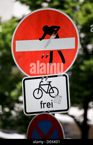
The first image might be difficult to classify because it is considerably covered from overgrown plants. Similarly images 2 and 3 also can be difficult to classify since they are covered with snow.
In addition to natural causes, traffic signs might also have defaced by people. Image 5 and 6 are examples of such cases where small patches of foreign items are sticked on the sign. However example 8 and 9 are some extreme cases where signs are defaced to the point of being almost unrecognizable.
Signs could also become difficult to classify due to being covered by shadows as in example 10 or as in example 11, being partially covered due to other objects in front of it when the sign is captured.
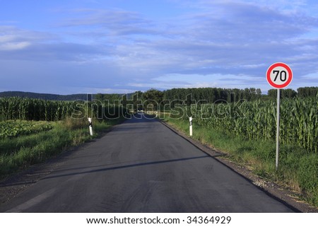
Twelfth image also might be difficult to classify since one of its feature is entirely faded out due to aging.
While skewed images like 13 and 14 could potentially make it hard to classify, convolutional neural networks are expected to cope up well with the smaller rotations or transformations in the images.
2. Discuss the model's predictions on these new traffic signs and compare the results to predicting on the test set. At a minimum, discuss what the predictions were, the accuracy on these new predictions, and compare the accuracy to the accuracy on the test set (OPTIONAL: Discuss the results in more detail as described in the "Stand Out Suggestions" part of the rubric).
Here are the results of the prediction:
| Image | Prediction |
|---|---|
| No entry | No entry |
| Road work | Road work |
| General caution | General caution |
| Road work | Road work |
| No entry | No entry |
| Ahead only | Ahead only |
| Priority road | Priority road |
| Stop | Priority road |
| Turn right ahead | Turn right ahead |
| Children crossing | Children crossing |
| Turn left ahead | Turn left ahead |
| Speed limit (70km/h) | Speed limit (70km/h) |
| General caution | General caution |
| Bumpy road | Bumpy road |
| Speed limit (70km/h) | Speed limit (70km/h) |
The model was able to correctly guess 14 of the 15 traffic signs, which gives an accuracy of 93.3%. This compares bit less favorably to the accuracy on the test set of 99.6%. However it should be noted that most of the traffic signs I have selected are defaced or otherwise not clear and difficult to classify.
Calculating the accuracy on these fifteen German traffic sign images found on the web might not give a comprehensive overview of how well the model is performing. One way to do a more detailed analysis of model performance is by looking at predictions in more detail. For this, I have calculated the precision and recall for each traffic sign type from the test set. Following diagrams shows precision and recall for each traffic sign type.
Recall:

Precision:

From these results, it is clear that model has a low recall for pedestrians signs. In other words, the model has trouble predicting on pedestrians signs. Probably we should generate more augment data for the pedestrians signs to help model generalize on pedestrians signs.
Also we can see that the model has low precision for pedestrians and no vehicles signs. In other words, if the model says something is a pedestrians or a no vehicles sign, we're not very sure that it really is a pedestrians or a no vehicles sign respectively. One possible reason for this could be due to the fact that there are some other types of traffic signs that are very similar to these types of traffic signs. Probably we could increase the model size a bit and see if things could be improved.
3. Describe how certain the model is when predicting on each of the five new images by looking at the softmax probabilities for each prediction. Provide the top 5 softmax probabilities for each image along with the sign type of each probability. (OPTIONAL: as described in the "Stand Out Suggestions" part of the rubric, visualizations can also be provided such as bar charts)
The code for making predictions on my final model is located in the 26th cell of the Ipython notebook.
Here I will discuss about how the model is predicting on few notable images.
For the first image, the model has relatively low confidence that this is a no entry sign (probability of 0.684), however the image does contain a no entry sign. The top five softmax probabilities were
| Probability | Prediction |
|---|---|
| 0.68441767 | No entry |
| 0.14791575 | Stop |
| 0.05323082 | Priority road |
| 0.011851982 | Yield |
| 0.0117532695 | No passing for vehicles over 3.5 metric tons |

For the second image also, the model has relatively low confidence that this is a road work sign (probability of 0.652), however the image does contain a road work sign even though it is considerably covered with snow. The top five softmax probabilities were
| Probability | Prediction |
|---|---|
| 0.652675 | Road work |
| 0.15080528 | Go straight or right |
| 0.04137244 | Bumpy road |
| 0.023628656 | Right-of-way at the next intersection |
| 0.019095229 | General caution |

Similarly for third image also model has very low confidence that this is a general caution sign (probability of 0.423), yet the image contains a general caution sign. The top five softmax probabilities were
| Probability | Prediction |
|---|---|
| 0.4230909 | General caution |
| 0.35896713 | Right-of-way at the next intersection |
| 0.075514 | Pedestrians |
| 0.03221925 | Go straight or left |
| 0.01742872 | Traffic signals |

Here one thing noticeable is that model has more or less equal score for the right of way at the next intersection sign as second most probable prediction. In fact these two signs are very much equal to each other graphically.
So it is safe to say that model is capable of handling cases where traffic sign is considerably covered with other objects. However we can see that confidence of the model is very low in such situations (It's quite amusing to see for the second image, model has come up with bumpy road as the 3rd guess which indeed would be the case with road works. And in fact road work sign contains a similar symbol to bumpy road symbol as part of it.)
However at this stage it should be stressed that the uncertainty of model predictions are due to the features of traffic sign being partially covered. Whereas model can confidently predict when traffic sign is clearer.
This is evident in fourth image, the model is quite certain that this is a road work sign (probability of 0.991), and the image does contain a road work sign. The top five softmax probabilities were
| Probability | Prediction |
|---|---|
| 0.991439 | Road work |
| 0.0025122187 | Keep left |
| 0.0015289161 | Go straight or right |
| 0.0008095841 | Stop |
| 0.00044973224 | General caution |

For the fifth image, the model is quite certain that this is a no entry sign (probability of 0.999), and the image does contain a no entry sign. The top five softmax probabilities were
| Probability | Prediction |
|---|---|
| 0.9992902 | No entry |
| 0.00045257795 | Stop |
| 2.2975235e-05 | Slippery road |
| 2.0329826e-05 | Children crossing |
| 1.9321327e-05 | Wild animals crossing |

This holds true for the case of sixth image where model is quite certain that it is ahead only sign (probability of 0.995), and the image does contain a ahead only sign.
For the eighth image, the model has low confidence in predicting that this is a priority road sign (probability of 0.541), however the image contains a seriously defaced stop sign. The top five softmax probabilities were
| Probability | Prediction |
|---|---|
| 0.54199773 | Priority road |
| 0.35776013 | Stop |
| 0.027231285 | No entry |
| 0.0099358 | Go straight or left |
| 0.009465913 | Ahead only |

It should be noted that this sign is quite defaced and indeed the 2nd prediction of the model is a stop sign with somewhat close confidence score (probability of 0.357).
For the ninth image also the model has very low confidence in predicting that it is turn right ahead sign (probability of 0.307), and the image does contain a turn right ahead sign. The top five softmax probabilities were
| Probability | Prediction |
|---|---|
| 0.3078608 | Turn right ahead |
| 0.25364423 | Roundabout mandatory |
| 0.16230176 | Keep left |
| 0.07043269 | Keep right |
| 0.034394156 | Pedestrians |

So despite the fact that the sign is defaced to the point that it is harder to identify by even human eye and easily could be mistaken to any of roundabout mandatory or keep left/right signs the model have somehow predicted the sign correctly. Here it seems that model is relying on overall background color to predict the class of signs and might have predicted the sign merely by coincidence.
For the tenth image, the model is quite certain that this is a children crossing sign (probability of 0.997), and the image does contain a children crossing sign. The top five softmax probabilities were
| Probability | Prediction |
|---|---|
| 0.9979644 | Children crossing |
| 0.00076279236 | Pedestrians |
| 0.00019365018 | Roundabout mandatory |
| 0.00018733578 | Speed limit (100km/h) |
| 0.0001830899 | Speed limit (30km/h) |

So despite being covered with some shadows, model is robust enough to predict the sign type correctly here.
For the eleventh image, the model has a moderate confidence that this is a turn left ahead sign (probability of 0.753), nevertheless the image does contain a partially occluded turn left ahead sign. The top five softmax probabilities were
| Probability | Prediction |
|---|---|
| 0.7538413 | Turn left ahead |
| 0.049201075 | Go straight or right |
| 0.00019365018 | Keep right |
| 0.03675174 | Priority road |
| 0.028343054 | Ahead only |

For the twelfth image, the model is quite certain that this is a speed limit (70km/h) sign (probability of 0.987), and the image does contain a speed limit (70km/h) sign. The top five softmax probabilities were
| Probability | Prediction |
|---|---|
| 0.98766553 | Speed limit (70km/h) |
| 0.0029435854 | Speed limit (30km/h) |
| 0.001769929 | Pedestrians |
| 0.00092452194 | Speed limit (20km/h) |
| 0.000903425 | Dangerous curve to the left |

So it is evident that even when a particular feature is completely absent or muted model is still capable of predicting based on the remaining features. It is quite interesting that the missing feature is indeed a common one to most of the classes that are confused. But it should be noted that a neural network may not necessarily create features as we look it but could be rather more complex higher dimensional features that are created by mix and match of segments of different segments of features we would normally see. (See below for a visualization of CNN activations.)
For the thirteenth image, the model is quite certain that this is a general caution sign (probability of 0.994), and the image does contain a general caution sign. The top five softmax probabilities were
| Probability | Prediction |
|---|---|
| 0.99483925 | General caution |
| 0.0010836464 | Pedestrians |
| 0.00061260955 | No entry |
| 0.0005754149 | Traffic signals |
| 0.00035156435 | Road narrows on the right |

As mentioned before convolutional neural networks are robust to rotations or transformations in image features. So model has no trouble classifying image 13 and 14 even though they are somewhat skewed due to the angle they were captured.
1. Discuss the visual output of your trained network's feature maps. What characteristics did the neural network use to make classifications?
Following image shows convolutional layer 1 activations of the DenseNet part of the model before and after training.
Untrained network:

Trained network:

From these visualizations it seems that neural network use some specific features in the images like color band around the traffic sign (For example see feature map 7) as well as some higher dimensional features comprising of parts of simple shapes and features represent in images. (For example see feature map 22)
When a particular feature from an image is not present, model could still perform with the remaining features of the image. For example when outer band of the above traffic sign is not present due to aging, the layers that solely depend on that feature seem to get less excited (For example see feature 7) whereas layers that either works as a combination of features or layers containing other features would contribute to make the model more robust. (For example see feature map 8, 9 and 18)
Trained network for an image with a feature missing:

However it should be noted that it's quite hard to explain how or why a neural network works with very complex models and images. Above is based on best explanation based on observations of the visualization of network.