Lab Exercise 2 is composed of three parts with several smaller parts. Write up your answers to all three parts as a GitHub flavored markdown file by the start of the next Lab on February 8, 2016.
Fossil species are recognized and classified on the basis of morphology. This introduces subjectivity into the process of classification because all species display some range of morphological variability and the line between intra- and interspecific variability is often a judgment call.
Click here to see illustrations of 25 ammonoid specimens. Your job will be to group them into species, keeping in mind the potential for intraspecific variability, ontogenetic change, and sexual dimorphism.
We are going to open the ammonite_classify.csv file in R. CSV stands for comma separated file, it is one of the most common file formats used in R for storing two-dimensional arrays - i.e., matrices or data frames. You can also view, create, and edit them using a spreadsheet program like Microsoft Excel.
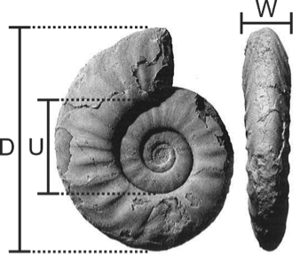
It is a data file containing shell coiling measurements traditionally used in ammonoid classification, including diameter (D), the ratio of umbilical width U to diameter (U/D), and the ratio of shell width W to diameter (W/D). The file also contains the stratigraphic position (relative geologic age) of each specimen.
To load the CSV file into R you will use the read.csv( ) function.
# First record the URL of the file as a character string - i.e., use quotes
URL<-"https://raw.githubusercontent.com/paleobiodb/teachPaleobiology/master/Lab2Figures/ammon_classify.csv"

# Save the CSV File as an object named Ammonites
# We will also use the row.names argument to tell R that the first column of the CSV file
# should be used as the rownames.
Ammonites<-read.csv(URL,row.names=1)Your basic workfow should be to first qualitatively (i.e., visually) decide which specimens you think belong to different species. Then you should subset the Ammonites array in R into several arrays based on your hypothesized species groupings. Using the techniques from the expertConcepts of the R tutorial (Lab 1), you can visualize, describe, or statistically test the different size and shape distributions of your hypothesized species.
You will find the following articles extremely helpful, particularly for question 4: An introducton to ammonites and Shell Anatomy and Diversity.
-
Your identifications (how many species do you recognize in the group, and which specimens belong to which species). Explain how and why you came to this conclusion.
-
The morphological features you used to distinguish each species, including whatever combination of qualitative or quantitative traits you think are important.
-
The nature of ontogenetic change, if any, in the species. Explain your reasoning.
-
The possibility of sexual dimorphism as a cause of morphological differences and how you evaluated that possibility.
We are going to perform a simple landmark analysis in R on pre-measured landmark data.
We will need to install an external package named geomorph into R. A package is a set of functions that another R user wrote and released for others to use. To install geomorph we will use the install.packages( ) function. You only ever need to do this step once per computer.
install.packages("geomorph")Some of you may recieve a prompt asking you to choose where you want to downlod the package from. You should ideally choose a location close to you, but it really doesn't matter.
You next need to activate the package. You only need to do installation (Step 1) once per computer, but you must load the package every new R session - i.e., every time you open R and want to use geomorph. You load packages using the library( ) function.
library(geomorph)The geomorph package comes with several pre-loaded example datasets. We are going to use two of these. hummingbirds and plethodon. Plethodons are a type of salamander.
# Load the example data in using the data( ) function
data(hummingbirds)
data(plethodon)
Take a look at the datasets. Notice that they are lists with several objects nested within them. Unfortunately, whoever made these datasets did not follow the first rule of R-club and it is fairly unclear what these objects are or mean. Let's do some ground-truthing using what you've learned about the properties of R objects.
-
Each element of the
plethodonlist has a name. What are they? -
What class is each object?
-
Whare are the dimensions of the first object in the plethodon list?
Based on the name, class, and structure of the first object in the plethodon list, we can surmise that it is a 3-dimensional array of morphometric landmark data. The first column represents x coordinates, the second column records y coordinates, and the third dimension represents different specimens.
This is the dataset we need to conduct a landmark analysis.
The first thing we need to do in a landmark analysis is a procrustes mathematical transformation. It takes its name from the ancient greek legend of Procrustes (Προκρούστης). Procrustes was a serial killer who would invite unsuspecting travellers to stay the night at his inn. If the travellers were too short for the bed, Procrustes would cruelly stretch out the travellers' bodies to fit the bed. If they were too tall for the bed, Procrustes would amputate their limbs until they fit.

Remember that landmark analysis is concerned with shape and not size. We therefore apply that the procrustes transformation to shrink or enlargen the data (specifically known as scaling) in such a way that we elminate size as a factor between specimens, but still maintain appropriate information about shape - i.e., the relative distance of the landmarks.
The mathematics behind this is fairly complex, but luckily there is a funciton in the geomorph packages that will do this for us. Let's perform a procrustes transformation on theplethodon landmarks using the gpagen( ) function.
ProcrustesPlethodon<-gpagen(plethodon[["land"]])The next step we need to do is a principle components analysis (PCA) on the transformed data. PCA is one of the most common forms of multivariate. A large part of this class will be about various forms of multivariate analyses. We will go more into the underlying theory of multivariate analyses - in general - in later labs. For now, we'll just explain the basic idea of PCA.
Because it can be used for a variety of purposes, not just morphometrics, there are several packages and functions for running a PCA in R. However, we will stick with the function built into the geomorph package, plotTangentSpace( ).
# plotTangentSpace both runs the PCA & plots it simultaneously. Other packages
# that we will use later in the semester will not do both of these things simulateneously
# so don't get confused. We are also going to turn of the warpgrids and verbose features,
# because we do not need them for our puproses.
plotTangentSpace(ProcrustesPlethodon[["coords"]],warpgrids=FALSE,verbose=FALSE)
Now that you have plotted the PCA, it should be obvious that the specimens cluster into three distinct morphologic groups based on their morphology - presumably this means that there are three different species in the data set. Though, remember, there can be other sources of morphologic variation.
-
Use the hummingbird dataset. Which object in the list records the landmark data?
-
Perform a procrustes on the landmark data.
-
Perform a PCA on the hummingbird data.
-
How many "species" of hummingbird are there?
Examine the following cladogram and answer the questions.

-
What is the synapomorphy of the clade containing species D and E?
-
What is a plesiomorphic character of that clade?
-
What is the synapomorphy of the clade containing species A and B?
-
Which taxa have a sulfurous odor?
-
What character distinguishes species D from species E?
-
Are adorable eyelashes a synapomorphy or an autapomorphy?
-
Traditionally, the five taxa are grouped into three families. Determine if each family is monophyletic, paraphyletic, or polyphyletic.
| Family | Species |
|---|---|
| Family 1 | Contains species A. |
| Family 2 | Contains species B and C. |
| Family 3 | contains species D and E. |
-
More recently, species A has been grouped in a family with species D and E. Is this advisable? Why or why not?
-
Determine if the following groups are monophyletic, paraphyletic, or polyphyletic.
| Group | Species |
|---|---|
| Group 1 | Species A, B, C. |
| Group 2 | Species C, D, E. |
| Group 3 | Species C and D. |
| Group 4 | Species A and B. |
| Group 5 | Species B, D, E. |
The following figure shows the pattern of shape change during ontogeny of the bivalve Gryphaea arcuata, from the early juvenile (A) to late juvenile (B) to adult (C). Note the magnification factors of the juvenile stages.

Here are adults of Gryphaea mccullochi (D) and Gryphaea gigantea (E). They are shown at x1.


https://raw.githubusercontent.com/paleobiodb/teachPaleobiology/master/Lab2Figures/ammon_classify.csv
The following figure shows the ontogeny of the trilobite Olenellus lapworthi (thin vertical arrow on left) and the evolutionary relationship of five species of Olenellus (large diagonal arrow).
-
Assuming that Gryphaea arcuata represents the ancestor, what type of heterochrony is most likely responsible for evolution of these two species?
-
Which species of Gryphaea has undergone a greater degree of heterochrony?
-
What type of heterochrony is represented in the Olenellus example??