Releases · PennyLaneAI/pennylane

28 Aug 17:15

v0.32.0

a9bc37a

Release 0.32.0

New features since last release

Encode matrices using a linear combination of unitaries ⛓️️

It is now possible to encode an operator A into a quantum circuit by decomposing it into a linear combination of unitaries using PREP (qml.StatePrep) and SELECT (qml.Select) routines. (#4431) (#4437) (#4444) (#4450) (#4506) (#4526)

Consider an operator A composed of a linear combination of Pauli terms:

>>> A = qml.PauliX(2) + 2 * qml.PauliY(2) + 3 * qml.PauliZ(2)

A decomposable block-encoding circuit can be created:

def block_encode(A, control_wires):
    probs = A.coeffs / np.sum(A.coeffs)
    state = np.pad(np.sqrt(probs, dtype=complex), (0, 1))
    unitaries = A.ops

    qml.StatePrep(state, wires=control_wires)
    qml.Select(unitaries, control=control_wires)
    qml.adjoint(qml.StatePrep)(state, wires=control_wires)

>>> print(qml.draw(block_encode, show_matrices=False)(A, control_wires=[0, 1]))
0: ─╭|Ψ⟩─╭Select─╭|Ψ⟩†─┤
1: ─╰|Ψ⟩─├Select─╰|Ψ⟩†─┤
2: ──────╰Select───────┤

This circuit can be used as a building block within a larger QNode to perform algorithms such as QSVT and Hamiltonian simulation.

Decomposing a Hermitian matrix into a linear combination of Pauli words via qml.pauli_decompose is now faster and differentiable. (#4395) (#4479) (#4493)

def find_coeffs(p):
    mat = np.array([[3, p], [p, 3]])
    A = qml.pauli_decompose(mat)
    return A.coeffs

>>> import jax
>>> from jax import numpy as np
>>> jax.jacobian(find_coeffs)(np.array(2.))
Array([0., 1.], dtype=float32, weak_type=True)

Monitor PennyLane's inner workings with logging 📃

Python-native logging can now be enabled with qml.logging.enable_logging(). (#4377) (#4383)

Consider the following code that is contained in my_code.py:

import pennylane as qml
qml.logging.enable_logging() # enables logging

dev = qml.device("default.qubit", wires=2)

@qml.qnode(dev)
def f(x):
    qml.RX(x, wires=0)
    return qml.state()

f(0.5)

Executing my_code.py with logging enabled will detail every step in PennyLane's pipeline that gets used to run your code.

$ python my_code.py
[1967-02-13 15:18:38,591][DEBUG][<PID 8881:MainProcess>] - pennylane.qnode.__init__()::"Creating QNode(func=<function f at 0x7faf2a6fbaf0>, device=<DefaultQubit device (wires=2, shots=None) at 0x7faf2a689b50>, interface=auto, diff_method=best, expansion_strategy=gradient, max_expansion=10, grad_on_execution=best, mode=None, cache=True, cachesize=10000, max_diff=1, gradient_kwargs={}"
...

Additional logging configuration settings can be specified by modifying the contents of the logging configuration file, which can be located by running qml.logging.config_path(). Follow our logging docs page for more details!

More input states for quantum chemistry calculations ⚛️

Input states obtained from advanced quantum chemistry calculations can be used in a circuit. (#4427) (#4433) (#4461) (#4476) (#4505)

Quantum chemistry calculations rely on an initial state that is typically selected to be the trivial Hartree-Fock state. For molecules with a complicated electronic structure, using initial states obtained from affordable post-Hartree-Fock calculations helps to improve the efficiency of the quantum simulations. These calculations can be done with external quantum chemistry libraries such as PySCF.

It is now possible to import a PySCF solver object in PennyLane and extract the corresponding wave function in the form of a state vector that can be directly used in a circuit. First, perform your classical quantum chemistry calculations and then use the qml.qchem.import_state function to import the solver object and return a state vector.
```
>>> from pyscf import gto, scf, ci
>>> mol = gto.M(atom=[['H', (0, 0, 0)], ['H', (0,0,0.71)]], basis='sto6g')
>>> myhf = scf.UHF(mol).run()
>>> myci = ci.UCISD(myhf).run()
>>> wf_cisd = qml.qchem.import_state(myci, tol=1e-1)
>>> print(wf_cisd)
[ 0.        +0.j  0.        +0.j  0.        +0.j  0.1066467 +0.j
  1.        +0.j  0.        +0.j  0.        +0.j  0.        +0.j
  2.        +0.j  0.        +0.j  0.        +0.j  0.        +0.j
 -0.99429698+0.j  0.        +0.j  0.        +0.j  0.        +0.j]
```
The state vector can be implemented in a circuit using qml.StatePrep.
```
>>> dev = qml.device('default.qubit', wires=4)
>>> @qml.qnode(dev)
... def circuit():
... qml.StatePrep(wf_cisd, wires=range(4))
... return qml.state()
>>> print(circuit())
[ 0.        +0.j  0.        +0.j  0.        +0.j  0.1066467 +0.j
  1.        +0.j  0.        +0.j  0.        +0.j  0.        +0.j
  2.        +0.j  0.        +0.j  0.        +0.j  0.        +0.j
 -0.99429698+0.j  0.        +0.j  0.        +0.j  0.        +0.j]
```
The currently supported post-Hartree-Fock methods are RCISD, UCISD, RCCSD, and UCCSD which denote restricted (R) and unrestricted (U) configuration interaction (CI) and coupled cluster (CC) calculations with single and double (SD) excitations.

Reuse and reset qubits after mid-circuit measurements ♻️

PennyLane now allows you to define circuits that reuse a qubit after a mid-circuit measurement has taken place. Optionally, the wire can also be reset to the $|0\rangle$ state. (#4402) (#4432)

Post-measurement reset can be activated by setting reset=True when calling qml.measure. In this version of PennyLane, executing circuits with qubit reuse will result in the defer_measurements transform being applied. This transform replaces each reused wire with an additional qubit. However, future releases of PennyLane will explore device-level support for qubit reuse without consuming additional qubits.

Qubit reuse and reset is also fully differentiable:
```
dev = qml.device("default.qubit", wires=4)

@qml.qnode(dev)
def circuit(p):
    qml.RX(p, wires=0)
    m = qml.measure(0, reset=True)
    qml.cond(m, qml.Hadamard)(1)

    qml.RX(p, wires=0)
    m = qml.measure(0)
    qml.cond(m, qml.Hadamard)(1)
    return qml.expval(qml.PauliZ(1))
```
```
>>> jax.grad(circuit)(0.4)
Array(-0.35867804, dtype=float32, weak_type=True)
```
You can read more about mid-circuit measurements in the documentation, and stay tuned for more mid-circuit measurement features in the next few releases!

Improvements 🛠

A new PennyLane drawing style

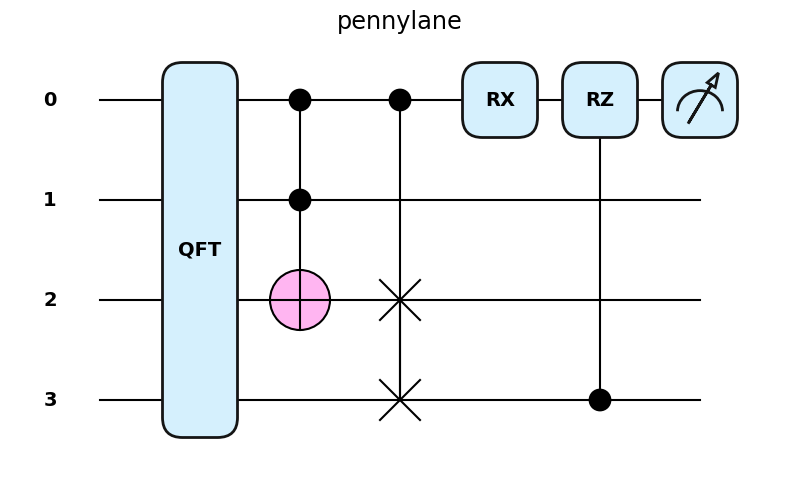
Circuit drawings and plots can now be created following a PennyLane style. (#3950)

The qml.draw_mpl function accepts a style='pennylane' argument to create PennyLane themed circuit diagrams:

def circuit(x, z):
    qml.QFT(wires=(0,1,2,3))
    qml.Toffoli(wires=(0,1,2))
    qml.CSWAP(wires=(0,2,3))
    qml.RX(x, wires=0)
    qml.CRZ(z, wires=(3,0))
    return qml.expval(qml.PauliZ(0))

qml.draw_mpl(circuit, style="pennylane")(1, 1)

PennyLane-styled plots can also be drawn by passing "pennylane.drawer.plot" to Matplotlib's plt.style.use function:

import matplotlib.pyplot as plt

plt.style.use("pennylane.drawer.plot")
for i in range(3):
    plt.plot(np.random.rand(10))

If the font Quicksand Bold isn't available, an available default font is used instead.

Making operators immutable and PyTrees

Any class inheriting from Operator is now automatically registered as a pytree with JAX. This unlocks the ability to jit functions of Operator. (#4458)

>>> op = qml.adjoint(qml.RX(1.0, wires=0))
>>> jax.jit(qml.matrix)(op)
Array([[0.87758255-0.j        , 0.        +0.47942555j],
       [0.        +0.47942555j, 0.87758255-0.j        ]],      dtype=complex64, weak_type=True)
>>> jax.tree_util.tree_map(lambd...

Assets 2

02 Aug 15:36

eddddddy

v0.31.1

0905217

Release 0.31.1

Improvements 🛠

data.Dataset now uses HDF5 instead of dill for serialization. (#4097)
The qchem functions primitive_norm and contracted_norm are modified to be compatible with higher versions of scipy. (#4321)

Bug Fixes 🐛

Dataset URLs are now properly escaped when fetching from S3. (#4412)

Contributors ✍️

This release contains contributions from (in alphabetical order):

Utkarsh Azad, Jack Brown, Diego Guala, Soran Jahangiri, Matthew Silverman

Assets 2

26 Jun 18:57

timmysilv

v0.31.0

18603e2

Release 0.31.0

New features since last release

Seamlessly create and combine fermionic operators 🔬

Fermionic operators and arithmetic are now available. (#4191) (#4195) (#4200) (#4201) (#4209) (#4229) (#4253) (#4255) (#4262) (#4278)

There are a couple of ways to create fermionic operators with this new feature:
- qml.FermiC and qml.FermiA: the fermionic creation and annihilation operators, respectively. These operators are defined by passing the index of the orbital that the fermionic operator acts on. For instance, the operators a⁺(0) and a(3) are respectively constructed as
```
>>> qml.FermiC(0)
a⁺(0)
>>> qml.FermiA(3)
a(3)
```
  These operators can be composed with (*) and linearly combined with (+ and -) other Fermi operators to create arbitrary fermionic Hamiltonians. Multiplying several Fermi operators together creates an operator that we call a Fermi word:
```
>>> word = qml.FermiC(0) * qml.FermiA(0) * qml.FermiC(3) * qml.FermiA(3)
>>> word 
a⁺(0) a(0) a⁺(3) a(3)
```
  Fermi words can be linearly combined to create a fermionic operator that we call a Fermi sentence:
```
>>> sentence = 1.2 * word - 0.345 * qml.FermiC(3) * qml.FermiA(3)
>>> sentence
1.2 * a⁺(0) a(0) a⁺(3) a(3)
- 0.345 * a⁺(3) a(3)
```
- via qml.fermi.from_string: create a fermionic operator that represents multiple creation and annihilation operators being multiplied by each other (a Fermi word).
```
>>> qml.fermi.from_string('0+ 1- 0+ 1-')
a⁺(0) a(1) a⁺(0) a(1)
>>> qml.fermi.from_string('0^ 1 0^ 1')
a⁺(0) a(1) a⁺(0) a(1)
```
  Fermi words created with from_string can also be linearly combined to create a Fermi sentence:
```
>>> word1 = qml.fermi.from_string('0+ 0- 3+ 3-')
>>> word2 = qml.fermi.from_string('3+ 3-')
>>> sentence = 1.2 * word1 + 0.345 * word2
>>> sentence
1.2 * a⁺(0) a(0) a⁺(3) a(3)
+ 0.345 * a⁺(3) a(3)
```
Additionally, any fermionic operator, be it a single fermionic creation/annihilation operator, a Fermi word, or a Fermi sentence, can be mapped to the qubit basis by using qml.jordan_wigner:
```
>>> qml.jordan_wigner(sentence)
((0.4725+0j)*(Identity(wires=[0]))) + ((-0.4725+0j)*(PauliZ(wires=[3]))) + ((-0.3+0j)*(PauliZ(wires=[0]))) + ((0.3+0j)*(PauliZ(wires=[0]) @ PauliZ(wires=[3])))
```
Learn how to create fermionic Hamiltonians describing some simple chemical systems by checking out our fermionic operators demo!

Workflow-level resource estimation 🧮

PennyLane's Tracker now monitors the resource requirements of circuits being executed by the device. (#4045) (#4110)

Suppose we have a workflow that involves executing circuits with different qubit numbers. We can obtain the resource requirements as a function of the number of qubits by executing the workflow with the Tracker context:

dev = qml.device("default.qubit", wires=4)

@qml.qnode(dev)
def circuit(n_wires):
    for i in range(n_wires):
        qml.Hadamard(i)
    return qml.probs(range(n_wires))

with qml.Tracker(dev) as tracker:
    for i in range(1, 5):
        circuit(i)

The resource requirements of individual circuits can then be inspected as follows:

>>> resources = tracker.history["resources"]
>>> resources[0]
wires: 1
gates: 1
depth: 1
shots: Shots(total=None)
gate_types:
{'Hadamard': 1}
gate_sizes:
{1: 1}
>>> [r.num_wires for r in resources]
[1, 2, 3, 4]

Moreover, it is possible to predict the resource requirements without evaluating circuits using the null.qubit device, which follows the standard execution pipeline but returns numeric zeros. Consider the following workflow that takes the gradient of a 50-qubit circuit:

n_wires = 50
dev = qml.device("null.qubit", wires=n_wires)

weight_shape = qml.StronglyEntanglingLayers.shape(2, n_wires)
weights = np.random.random(weight_shape, requires_grad=True)

@qml.qnode(dev, diff_method="parameter-shift")
def circuit(weights):
    qml.StronglyEntanglingLayers(weights, wires=range(n_wires))
    return qml.expval(qml.PauliZ(0))

with qml.Tracker(dev) as tracker:
    qml.grad(circuit)(weights)

The tracker can be inspected to extract resource requirements without requiring a 50-qubit circuit run:

>>> tracker.totals
{'executions': 451, 'batches': 2, 'batch_len': 451}
>>> tracker.history["resources"][0]
wires: 50
gates: 200
depth: 77
shots: Shots(total=None)
gate_types:
{'Rot': 100, 'CNOT': 100}
gate_sizes:
{1: 100, 2: 100}

Custom operations can now be constructed that solely define resource requirements — an explicit decomposition or matrix representation is not needed. (#4033)

PennyLane is now able to estimate the total resource requirements of circuits that include one or more of these operations, allowing you to estimate requirements for high-level algorithms composed of abstract subroutines.

These operations can be defined by inheriting from ResourcesOperation and overriding the resources() method to return an appropriate Resources object:

class CustomOp(qml.resource.ResourcesOperation):
    def resources(self):
        n = len(self.wires)
        r = qml.resource.Resources(
            num_wires=n,
            num_gates=n ** 2,
            depth=5,
        )
        return r

>>> wires = [0, 1, 2]
>>> c = CustomOp(wires)
>>> c.resources()
wires: 3
gates: 9
depth: 5
shots: Shots(total=None)
gate_types:
{}
gate_sizes:
{}

A quantum circuit that contains CustomOp can be created and inspected using qml.specs:

dev = qml.device("default.qubit", wires=wires)

@qml.qnode(dev)
def circ():
    qml.PauliZ(wires=0)
    CustomOp(wires)
    return qml.state()

>>> specs = qml.specs(circ)()
>>> specs["resources"].depth
6

Community contributions from UnitaryHack 🤝

ParametrizedHamiltonian now has an improved string representation. (#4176)

>>> def f1(p, t): return p[0] * jnp.sin(p[1] * t)
>>> def f2(p, t): return p * t
>>> coeffs = [2., f1, f2]
>>> observables =  [qml.PauliX(0), qml.PauliY(0), qml.PauliZ(0)]
>>> qml.dot(coeffs, observables)
  (2.0*(PauliX(wires=[0])))
+ (f1(params_0, t)*(PauliY(wires=[0])))
+ (f2(params_1, t)*(PauliZ(wires=[0])))

The quantum information module now supports trace distance. (#4181)

Two cases are enabled for calculating the trace distance:

A QNode transform via qml.qinfo.trace_distance:

dev = qml.device('default.qubit', wires=2)

@qml.qnode(dev)
def circuit(param):
    qml.RY(param, wires=0)
    qml.CNOT(wires=[0, 1])
    return qml.state()

>>> trace_distance_circuit = qml.qinfo.trace_distance(circuit, circuit, wires0=[0], wires1=[0])
>>> x, y = np.array(0.4), np.array(0.6)
>>> trace_distance_circuit((x,), (y,))
0.047862689546603415

Flexible post-processing via qml.math.trace_distance:

>>> rho = np.array([[0.3, 0], [0, 0.7]])
>>> sigma = np.array([[0.5, 0], [0, 0.5]])
>>> qml.math.trace_distance(rho, sigma)
0.19999999999999998

It is now possible to prepare qutrit basis states with qml.QutritBasisState. (#4185)

wires = range(2)
dev = qml.device("default.qutrit", wires=wires)

@qml.qnode(dev)
def qutrit_circuit():
    qml.QutritBasisState([1, 1], wires=wires)
    qml.TAdd(wires=wires)
    return qml.probs(wires=1)

>>> qutrit_circuit()
array([0., 0., 1.])

A new tra...

Assets 2

01 May 18:41

albi3ro

v0.30.0

4b4e693

Release 0.30.0

New features since last release

Pulse programming on hardware ⚛️🔬

Support for loading time-dependent Hamiltonians that are compatible with quantum hardware has been added, making it possible to load a Hamiltonian that describes an ensemble of Rydberg atoms or a collection of transmon qubits. (#3749) (#3911) (#3930) (#3936) (#3966) (#3987) (#4021) (#4040)

Rydberg atoms are the foundational unit for neutral atom quantum computing. A Rydberg-system Hamiltonian can be constructed from a drive term

qml.pulse.rydberg_drive — and an
interaction term
qml.pulse.rydberg_interaction:

from jax import numpy as jnp

atom_coordinates = [[0, 0], [0, 4], [4, 0], [4, 4]]
wires = [0, 1, 2, 3]
  
amplitude = lambda p, t: p * jnp.sin(jnp.pi * t)
phase = jnp.pi / 2
detuning = 3 * jnp.pi / 4

H_d = qml.pulse.rydberg_drive(amplitude, phase, detuning, wires)
H_i = qml.pulse.rydberg_interaction(atom_coordinates, wires)
H = H_d + H_i

The time-dependent Hamiltonian H can be used in a PennyLane pulse-level differentiable circuit:

dev = qml.device("default.qubit.jax", wires=wires)

@qml.qnode(dev, interface="jax")
def circuit(params):
    qml.evolve(H)(params, t=[0, 10])
    return qml.expval(qml.PauliZ(0))

>>> params = jnp.array([2.4])
>>> circuit(params)
Array(0.6316659, dtype=float32)
>>> import jax
>>> jax.grad(circuit)(params)
Array([1.3116529], dtype=float32)

The qml.pulse page contains additional details. Check out our release blog post for demonstration of how to perform the execution on actual hardware!

A pulse-level circuit can now be differentiated using a stochastic parameter-shift method. (#3780) (#3900) (#4000) (#4004)

The new qml.gradient.stoch_pulse_grad differentiation method unlocks stochastic-parameter-shift differentiation for pulse-level circuits. The current version of this new method is restricted to Hamiltonians composed of parametrized Pauli words, but future updates to extend to parametrized Pauli sentences can allow this method to be compatible with hardware-based systems such as an ensemble of Rydberg atoms.

This method can be activated by setting diff_method to qml.gradient.stoch_pulse_grad:

>>> dev = qml.device("default.qubit.jax", wires=2)
>>> sin = lambda p, t: jax.numpy.sin(p * t)
>>> ZZ = qml.PauliZ(0) @ qml.PauliZ(1)
>>> H = 0.5 * qml.PauliX(0) + qml.pulse.constant * ZZ + sin * qml.PauliX(1)
>>> @qml.qnode(dev, interface="jax", diff_method=qml.gradients.stoch_pulse_grad)
>>> def ansatz(params):
...     qml.evolve(H)(params, (0.2, 1.))
...     return qml.expval(qml.PauliY(1))
>>> params = [jax.numpy.array(0.4), jax.numpy.array(1.3)]
>>> jax.grad(ansatz)(params)
[Array(0.16921353, dtype=float32, weak_type=True),
 Array(-0.2537478, dtype=float32, weak_type=True)]

Quantum singular value transformation 🐛➡️🦋

PennyLane now supports the quantum singular value transformation (QSVT), which describes how a quantum circuit can be constructed to apply a polynomial transformation to the singular values of an input matrix. (#3756) (#3757) (#3758) (#3905) (#3909) (#3926) (#4023)

Consider a matrix A along with a vector angles that describes the target polynomial transformation. The qml.qsvt function creates a corresponding circuit:
```
dev = qml.device("default.qubit", wires=2)

A = np.array([[0.1, 0.2], [0.3, 0.4]])
angles = np.array([0.1, 0.2, 0.3])

@qml.qnode(dev)
def example_circuit(A):
    qml.qsvt(A, angles, wires=[0, 1])
    return qml.expval(qml.PauliZ(wires=0))
```
This circuit is composed of qml.BlockEncode and qml.PCPhase operations.
```
>>> example_circuit(A)
tensor(0.97777078, requires_grad=True)
>>> print(example_circuit.qtape.expand(depth=1).draw(decimals=2)) 
0: ─╭∏_ϕ(0.30)─╭BlockEncode(M0)─╭∏_ϕ(0.20)─╭BlockEncode(M0)†─╭∏_ϕ(0.10)─┤  <Z>
1: ─╰∏_ϕ(0.30)─╰BlockEncode(M0)─╰∏_ϕ(0.20)─╰BlockEncode(M0)†─╰∏_ϕ(0.10)─┤
```
The qml.qsvt function creates a circuit that is targeted at simulators due to the use of matrix-based operations. For advanced users, you can use the operation-based qml.QSVT template to perform the transformation with a custom choice of unitary and projector operations, which may be hardware compatible if a decomposition is provided.

The QSVT is a complex but powerful transformation capable of generalizing important algorithms like amplitude amplification. Stay tuned for a demo in the coming few weeks to learn more!

Intuitive QNode returns ↩️

An updated QNode return system has been introduced. PennyLane QNodes now return exactly what you tell them to! 🎉 (#3957) (#3969) (#3946) (#3913) (#3914) (#3934)

This was an experimental feature introduced in version 0.25 of PennyLane that was enabled via qml.enable_return(). Now, it's the default return system. Let's see how it works.

Consider the following circuit:
```
import pennylane as qml

dev = qml.device("default.qubit", wires=1)

@qml.qnode(dev)
def circuit(x):
    qml.RX(x, wires=0)
    return qml.expval(qml.PauliZ(0)), qml.probs(0)
```
In version 0.29 and earlier of PennyLane, circuit() would return a single length-3 array:
```
>>> circuit(0.5)
tensor([0.87758256, 0.93879128, 0.06120872], requires_grad=True)
```
In versions 0.30 and above, circuit() returns a length-2 tuple containing the expectation value and probabilities separately:
```
>>> circuit(0.5)
(tensor(0.87758256, requires_grad=True),
 tensor([0.93879128, 0.06120872], requires_grad=True))
```
You can find more details about this change, along with help and troubleshooting tips to solve any issues. If you still have questions, comments, or concerns, we encourage you to post on the PennyLane discussion forum.

A bunch of performance tweaks 🏃💨

Single-qubit operations that have multi-qubit control can now be decomposed more efficiently using fewer CNOT gates. (#3851)

Three decompositions from arXiv:2302.06377 are provided and compare favourably to the already-available qml.ops.ctrl_decomp_zyz:

wires = [0, 1, 2, 3, 4, 5]
control_wires = wires[1:]

@qml.qnode(qml.device('default.qubit', wires=6))
def circuit():
    with qml.QueuingManager.stop_recording():
        # the decomposition does not un-queue the target
        target = qml.RX(np.pi/2, wires=0)
    qml.ops.ctrl_decomp_bisect(target, (1,2,3,4,5))
    return qml.state()

print(qml.draw(circuit, expansion_strategy="device")())

0: ──H─╭X──U(M0)─╭X──U(M0)†─╭X──U(M0)─╭X──U(M0)†──H─┤  State
1: ────├●────────│──────────├●────────│─────────────┤  State
2: ────├●────────│──────────├●────────│─────────────┤  State
3: ────╰●────────│──────────╰●────────│─────────────┤  State
4: ──────────────├●───────────────────├●────────────┤  State
5: ──────────────╰●───────────────────╰●────────────┤  State

A new decomposition to qml.SingleExcitation has been added that halves the number of CNOTs required. (3976)

>>> qml.SingleExcitation.compute_decomposition(1.23, wires=(0,1))
[Adjoint(T(wires=[0])), Hadamard(wires=[0]), S(wires=[0]),...

Assets 2

06 Mar 17:16

albi3ro

v0.29.1

4b83860

Release v0.29.1

Bug fixes

Defines qml.math.ndim and qml.math.shape for builtins and autograd. Accommodates changes made by Autograd v0.6.1.

Contributors

This release contains contributions from (in alphabetical order):

Christina Lee

Assets 2

28 Feb 16:36

albi3ro

v0.29.0

5c13d41

Release 0.29.0

New features since last release

Pulse programming 🔊

Support for creating pulse-based circuits that describe evolution under a time-dependent Hamiltonian has now been added, as well as the ability to execute and differentiate these pulse-based circuits on simulator.
(#3586)(#3617)(#3645)(#3652)(#3665)(#3673)(#3706)(#3730)

A time-dependent Hamiltonian can be created using qml.pulse.ParametrizedHamiltonian, which holds information representing a linear combination of operators with parametrized coefficents and can be constructed as follows:

from jax import numpy as jnp

f1 = lambda p, t: p * jnp.sin(t) * (t - 1)
f2 = lambda p, t: p[0] * jnp.cos(p[1]* t ** 2)

XX = qml.PauliX(0) @ qml.PauliX(1)
YY = qml.PauliY(0) @ qml.PauliY(1)
ZZ = qml.PauliZ(0) @ qml.PauliZ(1)

H =  2 * ZZ + f1 * XX + f2 * YY

>>> H
ParametrizedHamiltonian: terms=3
>>> p1 = jnp.array(1.2)
>>> p2 = jnp.array([2.3, 3.4])
>>> H((p1, p2), t=0.5)
(2*(PauliZ(wires=[0]) @ PauliZ(wires=[1]))) + ((-0.2876553231625218*(PauliX(wires=[0]) @ PauliX(wires=[1]))) + (1.517961235535459*(PauliY(wires=[0]) @ PauliY(wires=[1]))))

The time-dependent Hamiltonian can be used within a circuit with qml.evolve:

def pulse_circuit(params, time):
    qml.evolve(H)(params, time)
    return qml.expval(qml.PauliX(0) @ qml.PauliY(1))

Pulse-based circuits can be executed and differentiated on the default.qubit.jax simulator using JAX as an interface:

>>> dev = qml.device("default.qubit.jax", wires=2)
>>> qnode = qml.QNode(pulse_circuit, dev, interface="jax")
>>> params = (p1, p2)
>>> qnode(params, time=0.5)
Array(0.72153819, dtype=float64)
>>> jax.grad(qnode)(params, time=0.5)
(Array(-0.11324919, dtype=float64),
 Array([-0.64399616,  0.06326374], dtype=float64))

Check out the qml.pulse documentation page for more details!

Special unitary operation 🌞

A new operation qml.SpecialUnitary has been added, providing access to an arbitrary unitary gate via a parametrization in the Pauli basis.
(#3650) (#3651) (#3674)

qml.SpecialUnitary creates a unitary that exponentiates a linear combination of all possible Pauli words in lexicographical order — except for the identity operator — for num_wires wires, of which there are 4**num_wires - 1. As its first argument, qml.SpecialUnitary takes a list of the 4**num_wires - 1 parameters that are the coefficients of the linear combination.

To see all possible Pauli words for num_wires wires, you can use the qml.ops.qubit.special_unitary.pauli_basis_strings function:
```
>>> qml.ops.qubit.special_unitary.pauli_basis_strings(1) # 4**1-1 = 3 Pauli words
['X', 'Y', 'Z']
>>> qml.ops.qubit.special_unitary.pauli_basis_strings(2) # 4**2-1 = 15 Pauli words
['IX', 'IY', 'IZ', 'XI', 'XX', 'XY', 'XZ', 'YI', 'YX', 'YY', 'YZ', 'ZI', 'ZX', 'ZY', 'ZZ']
```
To use qml.SpecialUnitary, for example, on a single qubit, we may define
```
>>> thetas = np.array([0.2, 0.1, -0.5])
>>> U = qml.SpecialUnitary(thetas, 0)
>>> qml.matrix(U)
array([[ 0.8537127 -0.47537233j,  0.09507447+0.19014893j],
       [-0.09507447+0.19014893j,  0.8537127 +0.47537233j]])
```
A single non-zero entry in the parameters will create a Pauli rotation:
```
>>> x = 0.412
>>> theta = x * np.array([1, 0, 0]) # The first entry belongs to the Pauli word "X"
>>> su = qml.SpecialUnitary(theta, wires=0)
>>> rx = qml.RX(-2 * x, 0) # RX introduces a prefactor -0.5 that has to be compensated
>>> qml.math.allclose(qml.matrix(su), qml.matrix(rx))
True
```
This operation can be differentiated with hardware-compatible methods like parameter shifts and it supports parameter broadcasting/batching, but not both at the same time. Learn more by visiting the qml.SpecialUnitary documentation.

Always differentiable 📈

The Hadamard test gradient transform is now available via qml.gradients.hadamard_grad. This transform is also available as a differentiation method within QNodes. (#3625) (#3736)

qml.gradients.hadamard_grad is a hardware-compatible transform that calculates the gradient of a quantum circuit using the Hadamard test. Note that the device requires an auxiliary wire to calculate the gradient.

>>> dev = qml.device("default.qubit", wires=2)
>>> @qml.qnode(dev)
... def circuit(params):
...     qml.RX(params[0], wires=0)
...     qml.RY(params[1], wires=0)
...     qml.RX(params[2], wires=0)
...     return qml.expval(qml.PauliZ(0))
>>> params = np.array([0.1, 0.2, 0.3], requires_grad=True)
>>> qml.gradients.hadamard_grad(circuit)(params)
(tensor(-0.3875172, requires_grad=True),
 tensor(-0.18884787, requires_grad=True),
 tensor(-0.38355704, requires_grad=True))

This transform can be registered directly as the quantum gradient transform to use during autodifferentiation:

>>> dev = qml.device("default.qubit", wires=2)
>>> @qml.qnode(dev, interface="jax", diff_method="hadamard")
... def circuit(params):
...     qml.RX(params[0], wires=0)
...     qml.RY(params[1], wires=0)
...     qml.RX(params[2], wires=0)
...     return qml.expval(qml.PauliZ(0))
>>> params = jax.numpy.array([0.1, 0.2, 0.3])
>>> jax.jacobian(circuit)(params)
Array([-0.3875172 , -0.18884787, -0.38355705], dtype=float32)

The gradient transform qml.gradients.spsa_grad is now registered as a differentiation method for QNodes.
(#3440)

The SPSA gradient transform can now be used implicitly by marking a QNode as differentiable with SPSA. It can be selected via
```
>>> dev = qml.device("default.qubit", wires=1)
>>> @qml.qnode(dev, interface="jax", diff_method="spsa", h=0.05, num_directions=20)
... def circuit(x):
...     qml.RX(x, 0)
...     return qml.expval(qml.PauliZ(0))
>>> jax.jacobian(circuit)(jax.numpy.array(0.5))
Array(-0.4792258, dtype=float32, weak_type=True)
```
The argument num_directions determines how many directions of simultaneous perturbation are used and therefore the number of circuit evaluations, up to a prefactor. See the SPSA gradient transform documentation for details. Note: The full SPSA optimization method is already available as qml.SPSAOptimizer.

The default interface is now auto. There is no need to specify the interface anymore; it is automatically determined by checking your QNode parameters.
(#3677)(#3752) (#3829)

import jax
import jax.numpy as jnp

qml.enable_return()
a = jnp.array(0.1)
b = jnp.array(0.2)

dev = qml.device("default.qubit", wires=2)

@qml.qnode(dev)
def circuit(a, b):
    qml.RY(a, wires=0)
    qml.RX(b, wires=1)
    qml.CNOT(wires=[0, 1])
    return qml.expval(qml.PauliZ(0)), qml.expval(qml.PauliY(1))

>>> circuit(a, b)
(Array(0.9950042, dtype=float32), Array(-0.19767681, dtype=float32))
>>> jac = jax.jacobian(circuit)(a, b)
>>> jac
(Array(-0.09983341, dtype=float32, weak_type=True), Array(0.01983384, dtype=float32, weak_type=True))

The JAX-JIT interface now supports higher-order gradient computation with the new return types system.
(#3498)

Here is an example of using JAX-JIT to compute the Hessian of a circuit:

import pennylane as qml
import jax
from jax import numpy as jnp

jax.config.update("jax_enable_x64", True)

qml.enable_return()

dev = qml.device("default.qubit", wires=2)

@jax.jit
@qml.qnode(dev, interface="jax-jit", diff_method="parameter-shift", max_diff=2)
def circuit(a, b):
    qml.RY(a, wires=0)
    qml.RX(b, wires=1)
    return qml.expval(qml.PauliZ(0)), qml.expval(qml.PauliZ(1))

a, b = jnp.array(1.0), jnp.array(2.0)

>>> jax.hessian(circuit, argnums=[0, 1])(a, b)
(((Array(-0.54030231, dtype=float64, weak_type=True),
   Array(0., dtype=float64, weak_type=True)),
  (Array(-1.76002563e-17, dtype=float64, weak_type=True),
   Array(0., dtype=float64, weak_type=True))),
 ((Array(0., dtype=float64, weak_type=True),
   Array(-1.00700085e-17, dtype=float64, weak_type=True)),
  (Array(0., dtype=float64, weak_type=True),
  Array(0.41614684, dtype=float64, weak_type=True))))

The qchem workflow has been modified to support both Autograd and JAX frameworks.
(#3458) (#3462) (#3495)

Th...

Assets 2

19 Dec 21:31

Jaybsoni

v0.28.0

568ac73

Release 0.28.0

New features since last release

Custom measurement processes 📐

Custom measurements can now be facilitated with the addition of the qml.measurements module. (#3286) (#3343) (#3288) (#3312) (#3287) (#3292) (#3287) (#3326) (#3327) (#3388) (#3439) (#3466)

Within qml.measurements are new subclasses that allow for the possibility to create custom measurements:
- SampleMeasurement: represents a sample-based measurement
- StateMeasurement: represents a state-based measurement
- MeasurementTransform: represents a measurement process that requires the application of a batch transform

Creating a custom measurement involves making a class that inherits from one of the classes above. An example is given below. Here, the measurement computes the number of samples obtained of a given state:

from pennylane.measurements import SampleMeasurement

class CountState(SampleMeasurement):
    def __init__(self, state: str):
        self.state = state  # string identifying the state, e.g. "0101"
        wires = list(range(len(state)))
        super().__init__(wires=wires)

    def process_samples(self, samples, wire_order, shot_range, bin_size):
        counts_mp = qml.counts(wires=self._wires)
        counts = counts_mp.process_samples(samples, wire_order, shot_range, bin_size)
        return counts.get(self.state, 0)

    def __copy__(self):
        return CountState(state=self.state)

We can now execute the new measurement in a QNode as follows.

dev = qml.device("default.qubit", wires=1, shots=10000)

@qml.qnode(dev)
def circuit(x):
    qml.RX(x, wires=0)
    return CountState(state="1")

>>> circuit(1.23)
tensor(3303., requires_grad=True)

Differentiability is also supported for this new measurement process:

>>> x = qml.numpy.array(1.23, requires_grad=True)
>>> qml.grad(circuit)(x)
4715.000000000001

For more information about these new features, see the documentation for qml.measurements.

ZX Calculus 🧮

QNodes can now be converted into ZX diagrams via the PyZX framework. (#3446)

ZX diagrams are the medium for which we can envision a quantum circuit as a graph in the ZX-calculus language, showing properties of quantum protocols in a visually compact and logically complete fashion.

QNodes decorated with @qml.transforms.to_zx will return a PyZX graph that represents the computation in the ZX-calculus language.

dev = qml.device("default.qubit", wires=2)

@qml.transforms.to_zx
@qml.qnode(device=dev)
def circuit(p):
    qml.RZ(p[0], wires=1),
    qml.RZ(p[1], wires=1),
    qml.RX(p[2], wires=0),
    qml.PauliZ(wires=0),
    qml.RZ(p[3], wires=1),
    qml.PauliX(wires=1),
    qml.CNOT(wires=[0, 1]),
    qml.CNOT(wires=[1, 0]),
    qml.SWAP(wires=[0, 1]),
    return qml.expval(qml.PauliZ(0) @ qml.PauliZ(1))

>>> params = [5 / 4 * np.pi, 3 / 4 * np.pi, 0.1, 0.3]
>>> circuit(params)
Graph(20 vertices, 23 edges)

Information about PyZX graphs can be found in the PyZX Graphs API.

QChem databases and basis sets ⚛️

The symbols and geometry of a compound from the PubChem database can now be accessed via qchem.mol_data(). (#3289) (#3378)

>>> import pennylane as qml
>>> from pennylane.qchem import mol_data
>>> mol_data("BeH2")
(['Be', 'H', 'H'],
 tensor([[ 4.79404621,  0.29290755,  0.        ],
              [ 3.77945225, -0.29290755,  0.        ],
              [ 5.80882913, -0.29290755,  0.        ]], requires_grad=True))
>>> mol_data(223, "CID")
(['N', 'H', 'H', 'H', 'H'],
 tensor([[ 0.        ,  0.        ,  0.        ],
              [ 1.82264085,  0.52836742,  0.40402345],
              [ 0.01417295, -1.67429735, -0.98038991],
              [-0.98927163, -0.22714508,  1.65369933],
              [-0.84773114,  1.373075  , -1.07733286]], requires_grad=True))

Perform quantum chemistry calculations with two new basis sets: 6-311g and CC-PVDZ. (#3279)

>>> symbols = ["H", "He"] 
>>> geometry = np.array([[1.0, 0.0, 0.0], [0.0, 0.0, 0.0]], requires_grad=False)
>>> charge = 1
>>> basis_names = ["6-311G", "CC-PVDZ"] 
>>> for basis_name in basis_names:
...     mol = qml.qchem.Molecule(symbols, geometry, charge=charge, basis_name=basis_name)
...     print(qml.qchem.hf_energy(mol)())
[-2.84429531] 
[-2.84061284]

A bunch of new operators 👀

The controlled CZ gate and controlled Hadamard gate are now available via qml.CCZ and qml.CH, respectively. (#3408)

>>> ccz = qml.CCZ(wires=[0, 1, 2])
>>> qml.matrix(ccz)
[[ 1  0  0  0  0  0  0  0]
 [ 0  1  0  0  0  0  0  0]
 [ 0  0  1  0  0  0  0  0]
 [ 0  0  0  1  0  0  0  0]
 [ 0  0  0  0  1  0  0  0]
 [ 0  0  0  0  0  1  0  0]
 [ 0  0  0  0  0  0  1  0]
 [ 0  0  0  0  0  0  0 -1]]
>>> ch = qml.CH(wires=[0, 1])
>>> qml.matrix(ch)
[[ 1.          0.          0.          0.        ]
 [ 0.          1.          0.          0.        ]
 [ 0.          0.          0.70710678  0.70710678]
 [ 0.          0.          0.70710678 -0.70710678]]

Three new parametric operators, qml.CPhaseShift00, qml.CPhaseShift01, and qml.CPhaseShift10, are now available. Each of these operators performs a phase shift akin to qml.ControlledPhaseShift but on different positions of the state vector. (#2715)

>>> dev = qml.device("default.qubit", wires=2)
>>> @qml.qnode(dev)
>>> def circuit():
...     qml.PauliX(wires=1)
...     qml.CPhaseShift01(phi=1.23, wires=[0,1])
...     return qml.state()
...
>>> circuit()
tensor([0.        +0.j       , 0.33423773+0.9424888j, 
        1.        +0.j       , 0.        +0.j       ], requires_grad=True)

A new gate operation called qml.FermionicSWAP has been added. This implements the exchange of spin orbitals representing fermionic-modes while maintaining proper anti-symmetrization. (#3380)

dev = qml.device('default.qubit', wires=2)

@qml.qnode(dev)
def circuit(phi):
    qml.BasisState(np.array([0, 1]), wires=[0, 1])
    qml.FermionicSWAP(phi, wires=[0, 1])
    return qml.state()

>>> circuit(0.1)
tensor([0.        +0.j        , 0.99750208+0.04991671j,
      0.00249792-0.04991671j, 0.        +0.j        ], requires_grad=True)

Create operators defined from a generator via qml.ops.op_math.Evolution. (#3375)

qml.ops.op_math.Evolution defines the exponential of an operator $\hat{O}$ of the form $e^{ix\hat{O}}$, with a single trainable parameter, $x$. Limiting to a single trainable parameter allows the use of qml.gradients.param_shift to find the gradient with respect to the parameter $x$.

dev = qml.device('default.qubit', wires=2)

@qml.qnode(dev, diff_method=qml.gradients.param_shift)
def circuit(phi):
    qml.ops.op_math.Evolution(qml.PauliX(0), -.5 * phi)
    return qml.expval(qml.PauliZ(0))

>>> phi = np.array(1.2)
>>> circuit(phi)
tensor(0.36235775, requires_grad=True)
>>> qml.grad(circuit)(phi)
-0.9320390495504149

The qutrit Hadamard gate, qml.THadamard, is now available. (#3340)

The operation accepts a subspace keyword argument which determines which variant of the qutrit Hadamard to use.

>>> th = qml.THadamard(wires=0, subspace=[0, 1])
>>> qml.matrix(th)
array([[ 0.70710678+0.j,  0.70710678+0.j,  0.        +0.j],
      [ 0.70710678+0.j, -0.70710678+0.j,  0.        +0.j],
      [ 0.        +0.j,  0.        +0.j,  1.        +0.j]])

New transforms, functions, and more 😯

Calculating the purity of arbitrary quantum states is now supported. (#3290)

The purity can be calculated in an analogous fashion to, say, the Von Neumann entropy:

qml.math.purity can be used as an in-line function:

>>> x = [1, 0, 0, 1] / np.sqrt(2)
>>> qml.math.purity(x, [0, 1])
1.0
>>> qml.math.purity(x, [0])
0.5

>>> x = [[1 / 2, 0, 0, 0], [0, 0, 0, 0], [0, 0, 0, 0], [0, 0, 0, 1 / 2]]
>>> qml.math.purity(x, [0, 1])
0.5

qml.qinfo.transforms.purity can transform a QNode returning a state to a
function that returns the purity:
```
dev = qml.device("default.mixed", wires=2)

@qml.qnode(dev)
de...
```

Assets 2

14 Nov 21:34

Jaybsoni

v0.27.0

51667d2

Release 0.27.0

New features since last release

An all-new data module 💾

The qml.data module is now available, allowing users to download, load, and create quantum datasets. (#3156)

Datasets are hosted on Xanadu Cloud and can be downloaded by using qml.data.load():

>>> H2_datasets = qml.data.load(
...   data_name="qchem", molname="H2", basis="STO-3G", bondlength=1.1
... )
>>> H2data = H2_datasets[0]
>>> H2data
<Dataset = description: qchem/H2/STO-3G/1.1, attributes: ['molecule', 'hamiltonian', ...]>

Datasets available to be downloaded can be listed with qml.data.list_datasets().

To download or load only specific properties of a dataset, we can specify the desired properties in qml.data.load with the attributes keyword argument:

>>> H2_hamiltonian = qml.data.load(
... data_name="qchem", molname="H2", basis="STO-3G", bondlength=1.1,
... attributes=["molecule", "hamiltonian"]
... )[0]
>>> H2_hamiltonian.hamiltonian
<Hamiltonian: terms=15, wires=[0, 1, 2, 3]>

The available attributes can be found using qml.data.list_attributes():

To select data interactively, we can use qml.data.load_interactive():

>>> qml.data.load_interactive()
Please select a data name:
    1) qspin
    2) qchem
Choice [1-2]: 1
Please select a sysname:
    ...
Please select a periodicity:
    ...
Please select a lattice:
    ...
Please select a layout:
    ...
Please select attributes:
    ...
Force download files? (Default is no) [y/N]: N
Folder to download to? (Default is pwd, will download to /datasets subdirectory):

Please confirm your choices:
dataset: qspin/Ising/open/rectangular/4x4
attributes: ['parameters', 'ground_states']
force: False
dest folder: datasets
Would you like to continue? (Default is yes) [Y/n]:
<Dataset = description: qspin/Ising/open/rectangular/4x4, attributes: ['parameters', 'ground_states']>

Once a dataset is loaded, its properties can be accessed as follows:

>>> dev = qml.device("default.qubit",wires=4)
>>> @qml.qnode(dev)
... def circuit():
...     qml.BasisState(H2data.hf_state, wires = [0, 1, 2, 3])
...     for op in H2data.vqe_gates:
...          qml.apply(op)
...     return qml.expval(H2data.hamiltonian)
>>> print(circuit())
-1.0791430411076344

It's also possible to create custom datasets with qml.data.Dataset:

>>> example_hamiltonian = qml.Hamiltonian(coeffs=[1,0.5], observables=[qml.PauliZ(wires=0),qml.PauliX(wires=1)])
>>> example_energies, _ = np.linalg.eigh(qml.matrix(example_hamiltonian))
>>> example_dataset = qml.data.Dataset(
... data_name = 'Example', hamiltonian=example_hamiltonian, energies=example_energies
... )
>>> example_dataset.data_name
'Example'
>>> example_dataset.hamiltonian
  (0.5) [X1]
+ (1) [Z0]
>>> example_dataset.energies
array([-1.5, -0.5,  0.5,  1.5])

Custom datasets can be saved and read with the qml.data.Dataset.write() and qml.data.Dataset.read() methods, respectively.

>>> example_dataset.write('./path/to/dataset.dat')
>>> read_dataset = qml.data.Dataset()
>>> read_dataset.read('./path/to/dataset.dat')
>>> read_dataset.data_name
'Example'
>>> read_dataset.hamiltonian
  (0.5) [X1]
+ (1) [Z0]
>>> read_dataset.energies
array([-1.5, -0.5,  0.5,  1.5])

We will continue to work on adding more datasets and features for qml.data in future releases.

Adaptive optimization 🏃🏋️🏊

Optimizing quantum circuits can now be done adaptively with qml.AdaptiveOptimizer. (#3192)

The qml.AdaptiveOptimizer takes an initial circuit and a collection of operators as input and adds a selected gate to the circuit at each optimization step. The process of growing the circuit can be repeated until the circuit gradients converge to zero within a given threshold. The adaptive optimizer can be used to implement algorithms such as ADAPT-VQE as shown in the following example.

Firstly, we define some preliminary variables needed for VQE:

symbols = ["H", "H", "H"]
geometry = np.array([[0.01076341, 0.04449877, 0.0],
                    [0.98729513, 1.63059094, 0.0],
                    [1.87262415, -0.00815842, 0.0]], requires_grad=False)
H, qubits = qml.qchem.molecular_hamiltonian(symbols, geometry, charge = 1)

The collection of gates to grow the circuit is built to contain all single and double excitations:

n_electrons = 2
singles, doubles = qml.qchem.excitations(n_electrons, qubits)
singles_excitations = [qml.SingleExcitation(0.0, x) for x in singles]
doubles_excitations = [qml.DoubleExcitation(0.0, x) for x in doubles]
operator_pool = doubles_excitations + singles_excitations

Next, an initial circuit that prepares a Hartree-Fock state and returns the expectation value of the Hamiltonian is defined:

hf_state = qml.qchem.hf_state(n_electrons, qubits)
dev = qml.device("default.qubit", wires=qubits)
@qml.qnode(dev)
def circuit():
    qml.BasisState(hf_state, wires=range(qubits))
    return qml.expval(H)

Finally, the optimizer is instantiated and then the circuit is created and optimized adaptively:

opt = qml.optimize.AdaptiveOptimizer()
for i in range(len(operator_pool)):
    circuit, energy, gradient = opt.step_and_cost(circuit, operator_pool, drain_pool=True)
    print('Energy:', energy)
    print(qml.draw(circuit)())
    print('Largest Gradient:', gradient)
    print()
    if gradient < 1e-3:
        break

Energy: -1.246549938420637
0: ─╭BasisState(M0)─╭G²(0.20)─┤ ╭<𝓗>
1: ─├BasisState(M0)─├G²(0.20)─┤ ├<𝓗>
2: ─├BasisState(M0)─│─────────┤ ├<𝓗>
3: ─├BasisState(M0)─│─────────┤ ├<𝓗>
4: ─├BasisState(M0)─├G²(0.20)─┤ ├<𝓗>
5: ─╰BasisState(M0)─╰G²(0.20)─┤ ╰<𝓗>
Largest Gradient: 0.14399872776755085

Energy: -1.2613740231529604
0: ─╭BasisState(M0)─╭G²(0.20)─╭G²(0.19)─┤ ╭<𝓗>
1: ─├BasisState(M0)─├G²(0.20)─├G²(0.19)─┤ ├<𝓗>
2: ─├BasisState(M0)─│─────────├G²(0.19)─┤ ├<𝓗>
3: ─├BasisState(M0)─│─────────╰G²(0.19)─┤ ├<𝓗>
4: ─├BasisState(M0)─├G²(0.20)───────────┤ ├<𝓗>
5: ─╰BasisState(M0)─╰G²(0.20)───────────┤ ╰<𝓗>
Largest Gradient: 0.1349349562423238

Energy: -1.2743971719780331
0: ─╭BasisState(M0)─╭G²(0.20)─╭G²(0.19)──────────┤ ╭<𝓗>
1: ─├BasisState(M0)─├G²(0.20)─├G²(0.19)─╭G(0.00)─┤ ├<𝓗>
2: ─├BasisState(M0)─│─────────├G²(0.19)─│────────┤ ├<𝓗>
3: ─├BasisState(M0)─│─────────╰G²(0.19)─╰G(0.00)─┤ ├<𝓗>
4: ─├BasisState(M0)─├G²(0.20)────────────────────┤ ├<𝓗>
5: ─╰BasisState(M0)─╰G²(0.20)────────────────────┤ ╰<𝓗>
Largest Gradient: 0.00040841755397108586

For a detailed breakdown of its implementation, check out the Adaptive circuits for quantum chemistry demo.

Automatic interface detection 🧩

QNodes now accept an auto interface argument which automatically detects the machine learning library to use. (#3132)

from pennylane import numpy as np
import torch
import tensorflow as tf
from jax import numpy as jnp

dev = qml.device("default.qubit", wires=2)
@qml.qnode(dev, interface="auto")
def circuit(weight):
    qml.RX(weight[0], wires=0)
    qml.RY(weight[1], wires=1)
    return qml.expval(qml.PauliZ(0))

interface_tensors = [[0, 1], np.array([0, 1]), torch.Tensor([0, 1]), tf.Variable([0, 1], dtype=float), jnp.array([0, 1])]
for tensor in interface_tensors:
    res = circuit(weight=tensor)
    print(f"Result value: {res:.2f}; Result type: {type(res)}")

Result value: 1.00; Result type: <class 'pennylane.numpy.tensor.tensor'>
Result value: 1.00; Result type: <class 'pennylane.numpy.tensor.tensor'>
Result value: 1.00; Result type: <class 'torch.Tensor'>
Result value: 1.00; Result type: <class 'tensorflow.python.framework.ops.EagerTensor'>
Result value: 1.00; Result type: <class 'jaxlib.xla_extension.DeviceArray'>

Upgraded JAX-JIT gradient support 🏎

JAX-JIT support for computing the gradient of QNodes that return a single vector of probabilities or multiple expectation values is now available. (#3244) (#3261)

import jax
from jax import numpy as jnp
from jax.config import config
config.update("jax_enable_x64", True)

dev = qml.device("lightning.qubit", wires=2)

@jax.jit
@qml.qnode(dev, diff_method="parameter-shift", interface="jax")
def circuit(x, y):
    qml.RY(x, wires=0)
    qml.RY(y, wires=1)
    qml.CNOT(wires=[0, 1])
    return qml.expval(qml.PauliZ(0)), qml.expval(qml.PauliZ(1))

x = jnp.array(1.0)
y = jnp.array(2.0)

>>> jax.jacobian(circuit, argnums=[0, 1])(x, y)
(DeviceArray([-0.84147098,  0.35017549], dtype=float64, weak_type=True),
 DeviceArray([ 4.47445479e-18, -4.91295496e-01], dtype=float64, weak_type=True))

Note that this change depends on jax.pure_callback, which requires jax>=0.3.17.

Construct Pauli words and sentences 🔤

We've reorganized and grouped everything in PennyLane responsible for manipulating Pauli operators into a pauli module. The grouping module has been deprecated as a result, and logic was moved from pennylane/grouping to `pe...

Assets 2

26 Sep 20:10

josh146

v0.26.0-postfix-1

2ebd0e0

Release 0.26.0-postfix1

A minor postfix release to update the documentation styling.

Assets 2

19 Sep 17:48

rmoyard

v0.26.0

18aeaf6

Release 0.26.0

New features since last release

Classical shadows 👤

PennyLane now provides built-in support for implementing the classical-shadows measurement protocol. (#2820) (#2821) (#2871) (#2968) (#2959) (#2968)

The classical-shadow measurement protocol is described in detail in the paper Predicting Many Properties of a Quantum System from Very Few Measurements. As part of the support for classical shadows in this release, two new finite-shot and fully-differentiable measurements are available:
- QNodes returning the new measurement qml.classical_shadow() will return two entities; bits (0 or 1 if the 1 or -1 eigenvalue is sampled, respectively) and recipes (the randomized Pauli measurements that are performed for each qubit, labelled by integer):
```
dev = qml.device("default.qubit", wires=2, shots=3)

@qml.qnode(dev)
def circuit():
    qml.Hadamard(wires=0)
    qml.CNOT(wires=[0, 1])
    return qml.classical_shadow(wires=[0, 1])
```
```
>>> bits, recipes = circuit()
>>> bits
tensor([[0, 0],
        [1, 0],
        [0, 1]], dtype=uint8, requires_grad=True)
>>> recipes
tensor([[2, 2],
        [0, 2],
        [0, 2]], dtype=uint8, requires_grad=True)
```
- QNodes returning qml.shadow_expval() yield the expectation value estimation using classical shadows:
```
dev = qml.device("default.qubit", wires=range(2), shots=10000)

@qml.qnode(dev)
def circuit(x, H):
    qml.Hadamard(0)
    qml.CNOT((0,1))
    qml.RX(x, wires=0)
    return qml.shadow_expval(H)

x = np.array(0.5, requires_grad=True) 
H = qml.Hamiltonian(
        [1., 1.], 
        [qml.PauliZ(0) @ qml.PauliZ(1), qml.PauliX(0) @ qml.PauliX(1)]
    )  
```
```
>>> circuit(x, H)
tensor(1.8486, requires_grad=True) 
>>> qml.grad(circuit)(x, H)
-0.4797000000000001
```
Fully-differentiable QNode transforms for both new classical-shadows measurements are also available via qml.shadows.shadow_state and qml.shadows.shadow_expval, respectively.

For convenient post-processing, we've also added the ability to calculate general Renyi entropies by way of the ClassicalShadow class' entropy method, which requires the wires of the subsystem of interest and the Renyi entropy order:
```
>>> shadow = qml.ClassicalShadow(bits, recipes)
>>> vN_entropy = shadow.entropy(wires=[0, 1], alpha=1)
```

Qutrits: quantum circuits for tertiary degrees of freedom ☘️

An entirely new framework for quantum computing is now simulatable with the addition of qutrit functionalities. (#2699) (#2781) (#2782) (#2783) (#2784) (#2841) (#2843)

Qutrits are like qubits, but instead live in a three-dimensional Hilbert space; they are not binary degrees of freedom, they are tertiary. The advent of qutrits allows for all sorts of interesting theoretical, practical, and algorithmic capabilities that have yet to be discovered.

To facilitate qutrit circuits requires a new device: default.qutrit. The default.qutrit device is a Python-based simulator, akin to default.qubit, and is defined as per usual:
```
>>> dev = qml.device("default.qutrit", wires=1)
```
The following operations are supported on default.qutrit devices:
- The qutrit shift operator, qml.TShift, and the ternary clock operator, qml.TClock, as defined in this paper by Yeh et al. (2022),
  which are the qutrit analogs of the Pauli X and Pauli Z operations, respectively.
- The qml.TAdd and qml.TSWAP operations which are the qutrit analogs of the CNOT and SWAP operations, respectively.
- Custom unitary operations via qml.QutritUnitary.
- qml.state and qml.probs measurements.
- Measuring user-specified Hermitian matrix observables via qml.THermitian.
A comprehensive example of these features is given below:
```
dev = qml.device("default.qutrit", wires=1)

U = np.array([
        [1, 1, 1], 
        [1, 1, 1], 
        [1, 1, 1]
    ]
) / np.sqrt(3) 

obs = np.array([
        [1, 1, 0], 
        [1, -1, 0], 
        [0, 0, np.sqrt(2)]
    ]
) / np.sqrt(2)

@qml.qnode(dev)
def qutrit_state(U, obs):
    qml.TShift(0)
    qml.TClock(0)
    qml.QutritUnitary(U, wires=0)
    return qml.state()

@qml.qnode(dev)
def qutrit_expval(U, obs):
    qml.TShift(0)
    qml.TClock(0)
    qml.QutritUnitary(U, wires=0)
    return qml.expval(qml.THermitian(obs, wires=0))
```
```
>>> qutrit_state(U, obs)
tensor([-0.28867513+0.5j, -0.28867513+0.5j, -0.28867513+0.5j], requires_grad=True) 
>>> qutrit_expval(U, obs)
tensor(0.80473785, requires_grad=True)
```
We will continue to add more and more support for qutrits in future releases.

Simplifying just got... simpler 😌

The qml.simplify() function has several intuitive improvements with this release. (#2978) (#2982) (#2922) (#3012)

qml.simplify can now perform the following:
- simplify parametrized operations
- simplify the adjoint and power of specific operators
- group like terms in a sum
- resolve products of Pauli operators
- combine rotation angles of identical rotation gates
Here is an example of qml.simplify in action with parameterized rotation gates. In this case, the angles of rotation are simplified to be modulo $4\pi$.
```
>>> op1 = qml.RX(30.0, wires=0)
>>> qml.simplify(op1)
RX(4.867258771281655, wires=[0])
>>> op2 = qml.RX(4 * np.pi, wires=0)
>>> qml.simplify(op2)
Identity(wires=[0])
```
All of these simplification features can be applied directly to quantum functions, QNodes, and tapes via decorating with @qml.simplify, as well:
```
dev = qml.device("default.qubit", wires=2)
@qml.simplify
@qml.qnode(dev)
def circuit():
    qml.adjoint(qml.prod(qml.RX(1, 0) ** 1, qml.RY(1, 0), qml.RZ(1, 0)))
    return qml.probs(wires=0)
```
```
>>> circuit()
>>> list(circuit.tape)
[RZ(11.566370614359172, wires=[0]) @ RY(11.566370614359172, wires=[0]) @ RX(11.566370614359172, wires=[0]),
 probs(wires=[0])]
```

QNSPSA optimizer 💪

A new optimizer called qml.QNSPSAOptimizer is available that implements the quantum natural simultaneous perturbation stochastic approximation (QNSPSA) method based on Simultaneous Perturbation Stochastic Approximation of the Quantum Fisher Information. (#2818)

qml.QNSPSAOptimizer is a second-order SPSA algorithm, which combines the convergence power of the quantum-aware Quantum Natural Gradient (QNG) optimization method with the reduced quantum evaluations of SPSA methods.

While the QNSPSA optimizer requires additional circuit executions (10 executions per step) compared to standard SPSA optimization (3 executions per step), these additional evaluations are used to provide a stochastic estimation of a second-order metric tensor, which often helps the optimizer to achieve faster convergence.

Use qml.QNSPSAOptimizer like you would any other optimizer:
```
max_iterations = 50
opt = qml.QNSPSAOptimizer() 

for _ in range(max_iterations):
    params, cost = opt.step_and_cost(cost, params)
```
Check out our demo on the QNSPSA optimizer for more information.

Operator and parameter broadcasting supplements 📈

Operator methods for exponentiation and raising to a power have been added. (#2799) (#3029)

The qml.exp function can be used to create observables or generic rotation gates:

>>> x = 1.234
>>> t = qml.PauliX(0) @ qml.PauliX(1) + qml.PauliY(0) @ qml.PauliY(1)
>>> isingxy = qml.exp(t, 0.25j * x)
>>> isingxy.matrix()
array([[1.       +0.j        , 0.       +0.j        ,
    1.       +0.j        , 0.       +0.j        ],
   [0.       +0.j        , 0.8156179+0.j        ,
    1.       +0.57859091j, 0.       +0.j        ],
   [0.       +0.j        , 0.       +0.57859091j,
    0.8156179+0.j        , 0.       +0.j        ],
   [0.       +0.j        , 0.       +0.j        ,
    1.       +0.j        , 1.       +0.j        ]])

The qml.pow function raises a given operator to a power:

>>> op = qml.pow(qml.PauliX(0), 2)
>>> op.matrix()
array([[1, 0], [0, 1]])

An operat...

Assets 2

Releases: PennyLaneAI/pennylane

Release 0.32.0

New features since last release

Encode matrices using a linear combination of unitaries ⛓️️

Monitor PennyLane's inner workings with logging 📃

More input states for quantum chemistry calculations ⚛️

Reuse and reset qubits after mid-circuit measurements ♻️

Improvements 🛠

A new PennyLane drawing style

Making operators immutable and PyTrees

Release 0.31.1

Improvements 🛠

Bug Fixes 🐛

Contributors ✍️

Release 0.31.0

New features since last release

Seamlessly create and combine fermionic operators 🔬

Workflow-level resource estimation 🧮

Community contributions from UnitaryHack 🤝

Release 0.30.0

New features since last release

Pulse programming on hardware ⚛️🔬

Quantum singular value transformation 🐛➡️🦋

Intuitive QNode returns ↩️

A bunch of performance tweaks 🏃💨

Release v0.29.1

Bug fixes

Contributors

Release 0.29.0

New features since last release

Pulse programming 🔊

Special unitary operation 🌞

Always differentiable 📈

Release 0.28.0

New features since last release

Custom measurement processes 📐

ZX Calculus 🧮

QChem databases and basis sets ⚛️

A bunch of new operators 👀

New transforms, functions, and more 😯

Release 0.27.0

New features since last release

An all-new data module 💾

Adaptive optimization 🏃🏋️🏊

Automatic interface detection 🧩

Upgraded JAX-JIT gradient support 🏎

Construct Pauli words and sentences 🔤

Release 0.26.0-postfix1

Release 0.26.0

New features since last release

Classical shadows 👤

Qutrits: quantum circuits for tertiary degrees of freedom ☘️

Simplifying just got... simpler 😌

QNSPSA optimizer 💪

Operator and parameter broadcasting supplements 📈