Clarification on issues experience with Adjoint Simulations in Meep #1896
Replies: 12 comments 4 replies
-
|
For this particular problem, the objective function seems to involve focusing the fields within a homogeneous medium (i.e., free space) rather than maximizing transmission into a guided mode (as in the tutorial example you referenced involving the power splitter). You should therefore be using the (Separately, we will soon be revamping the tutorials for the adjoint solver since currently many of them are out of date.) |
Beta Was this translation helpful? Give feedback.
-
|
Thanks @oskooi I appreciate the help! I will make the changes and see if I can get this working. I'll leave this issue open for now until I have tested them but will close if they work. |
Beta Was this translation helpful? Give feedback.
-
|
Here's a few suggestions I have:
sources = [mp.EigenmodeSource(mp.GaussianSource(fcen=f,fwidth=0.2*f),<<other args here>>) for f in [1/0.5, 1/0.6]]This is actually better because the mode profile is computed at each frequency of interest. If you try to do a single source, the spatial profile is only calculated at the center frequency, and you could see some errors from mode dispersion.
(edit: fixed |
Beta Was this translation helpful? Give feedback.
-
|
@smartalecH thanks for the help! I have made these adjustments to the simulation but is seems that by changing the sources to a ContinuousSource the simulation never completes 1 forward run of the adjoint method. I am assuming that is because I have tried to make the suggested changes, leaving me with my objective functions as: the And the cost function passed to the This runs fine for the forward runs and seems to calculate the gradient in the I am not sure if this is an issue with how I am setting up |
Beta Was this translation helpful? Give feedback.
-
Whoops! Sorry, I meant multiple Recall that a |
Beta Was this translation helpful? Give feedback.
-
Your objective function is currently outputting two values (multi-objective). You either need to do an epigraph (see the tutorials) or sum your objective so that it's scalar-valued (note this is not unique to meep, but rather an intrinsic characteristic of multi-objective optimization). For example, if you opt for the scalar-valued approach, you could simply do: def J(source, top, bottom):
return npa.mean(npa.abs(top[0] ** 2) / npa.abs(source[0] ** 2)) + npa.mean(npa.abs(bottom[1] ** 2) / npa.abs(source[1] ** 2))If you opt for the epigraph, make sure you take care of the gradient array properly (again, discussed in the above-linked tutorial). |
Beta Was this translation helpful? Give feedback.
-
|
@smartalecH I had tried that as my objective function before I posted my reply but ran into: I know that the objective needs to be scalar valued, but I thought by outputting two values they would be interpreted as the objective functions for each frequency. I must have been interpreting this incorrectly But then I run into the same error: When calling I am currently using the Meep version available through anaconda (1, 2.1) if that might be an issue, I havn't inspected the changes between that and the current master version. |
Beta Was this translation helpful? Give feedback.
-
|
Have tried the epigraph formulation. When I dont try normalize by the source power, the density doesn't change at all. If I do include some normalization to J it is a little bit better, at least there looks to be change in the density But the there splitting of the 500(top) and 700nm(bottom) wavelength light. If I try go for just a scalar value for J: I run into I know the tutorials are out-dated but just as an FYI this occurs in the I have also tried various other way of handling the gradients when using an objective function where I do not take the mean and thus am able to get the adjoint simulation working when there are multiple frequencies: But I have had no luck for the different ways I've tried handling these gradients in Any advice would be greatly appreciated. |
Beta Was this translation helpful? Give feedback.
-
|
The objective function import meep as mp
import meep.adjoint as mpa
import numpy as np
from autograd import numpy as npa
Si = mp.Medium(index=3.5)
resolution = 20 # pixels/μm
wvl_min = 0.4
wvl_max = 0.7
frq_min = 1/wvl_max
frq_max = 1/wvl_min
fcen = 0.5*(frq_min+frq_max)
df = frq_max-frq_min
nfreqs = 21
freqs = 1/np.linspace(wvl_min, wvl_max, nfreqs)
dpml = 0.5*wvl_max
dair = wvl_max
dfocus = 2.0 # focal distance from the nearest edge of the filter
design_region_shape = mp.Vector3(1.,2.,0)
sx = dpml + dair + design_region_shape.x + dfocus + dair + dpml
sy = dpml + design_region_shape.y + dpml
cell_size = mp.Vector3(sx,sy)
pml_layers = [mp.PML(dpml)]
source = [mp.Source(mp.GaussianSource(frequency=fcen,fwidth=df,is_integrated=True),
size=mp.Vector3(0,sy,0),
center=mp.Vector3(-0.5*sx+dpml),
component=mp.Ez)]
design_region_resolution = 2*resolution
Nx = int(design_region_shape.x*design_region_resolution) + 1
Ny = int(design_region_shape.y*design_region_resolution) + 1
design_variables = mp.MaterialGrid(mp.Vector3(Nx,Ny),
mp.air,
Si,
weights=np.ones((Nx,Ny)))
design_region_center = mp.Vector3(x=-0.5*sx+dpml+dair+0.5*design_region_shape.x)
design_region = mpa.DesignRegion(design_variables,
volume=mp.Volume(center=design_region_center,
size=design_region_shape))
geometry = [
mp.Block(center=design_region_center,
size=design_region_shape,
material=design_variables)
]
sim = mp.Simulation(cell_size=cell_size,
boundary_layers=pml_layers,
geometry=geometry,
sources=source,
k_point=mp.Vector3(),
resolution=resolution)
# line monitor for the DFT fields at the focal distance
ob_list = [mpa.FourierFields(sim,
mp.Volume(center=mp.Vector3(x=0.5*sx-dpml-dair),
size=mp.Vector3(y=sy-2*dpml)),
component=mp.Ez)]
# scalar objective function for maximizing
# Ez intensity at a given frequency and spatial point
# of the DFT line monitor while minimizing Ez intensity
# at all other frequencies at that same point
def J(mon):
frq_idx = 5
pt_idx = 10
intensity = npa.concatenate((-1*npa.power(npa.abs(mon[:frq_idx,pt_idx]),2),
[npa.power(npa.abs(mon[frq_idx,pt_idx]),2)],
-1*npa.power(npa.abs(mon[frq_idx+1:,pt_idx]),2)))
return intensity
opt = mpa.OptimizationProblem(
simulation=sim,
objective_functions=J,
objective_arguments=ob_list,
design_regions=[design_region],
frequencies=freqs,
maximum_run_time=100,
)
x0 = 0.5*np.ones((Nx*Ny,))
val, grad = opt([x0])
print(f"{val.shape}, {grad.shape}")output |
Beta Was this translation helpful? Give feedback.
-
|
If I get time this week, I'll try throwing together a tutorial that can design this structure. |
Beta Was this translation helpful? Give feedback.
-
|
For your reference, a manuscript describing the inner workings of Meep's adjoint solver was published today in Optics Express: https://opg.optica.org/oe/fulltext.cfm?uri=oe-30-3-4467&id=468836. |
Beta Was this translation helpful? Give feedback.
-
|
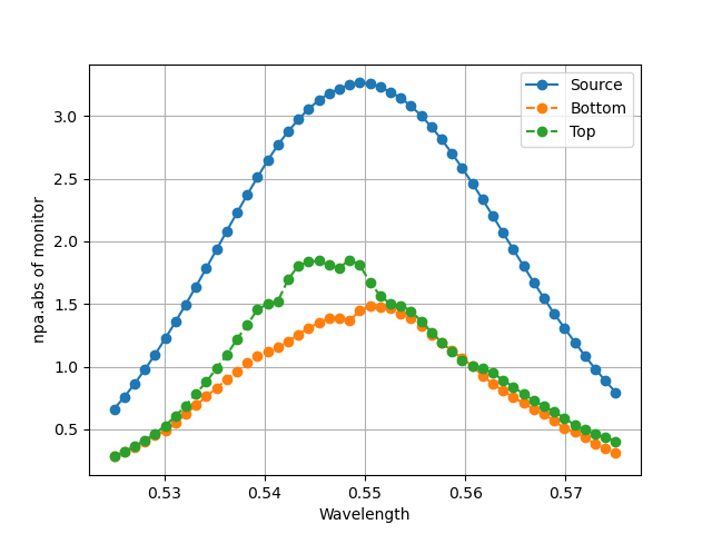
I have some updates and additional questions: Epigraph formulation seems to starting to bear fruit for what I want to do. I get results that at least show that the ratio of power from source to the desired focus point (my figure of merit) is driven in the correct direction. This is the plot of the sum of the absolute values of the fields (using a The top monitor is a focus for the first 6 frequencies points and bottom monitor for the next 6. On closer inspection if I look at the fields at the monitors I see that what actually seems to be happening is that the power measured at the source monitor I suspect that this is because the figure of merit normalizes by the source monitors power, so an effective means of increasing the FOM is to reduce the power at the source monitor, so the device structure that results from this optimization does some focusing of the power between the top and bottom monitors, but also trys to have a lot of destructive interference at the source monitor (via reflections off the device) to minimize the source power. Is there a way to avoid this? I have tried to remove the source term normalization in the calculation, without much success, I am not sure if I formulated the epigraph problem correctly in this case I changed it from minimization (FOM=1-monitor_power/source_power) to a maximization problem (FOM=monitor_power), but this does not seem to correspond to a well formed minimax problem. I still need to do some more research into this type of optimization. I also would like to know if I want to make lenses that focus power onto a specific region is it better to sum the power over all points in that region or would taking the power just at the central location be a good enough solution? It would seem that over the whole field would be optimal. In preliminary testing it seemed that it did not work as well, but that could be because I messed up the epigraph formalization when making it a maximization problem. One thing I did notice was that it was much faster when only optimizing one point. What is the correct way to start/restart a optimization? Do I use the dump_structure and load_structure functions? Do I save the opt.design_regions design_parameters.weights? How do I look at the actual values of the dielectric? I see that according to the paper referenced by @oskooi they get interpolated but when I look at opt.design_regions[0].design_parameters.weights they are all much higher values than my materials dielectric constant/index of refraction. Do I use The source monitor seems to be non-uniform, could this be because I am placing my sources incorrectly? @smartalecH's comment suggests that I use multiple sources, Is there a good rule of thumb for how many to use? I tried to use 3 sources and space them so their full width at half max values values coincided with one another. without much success. I tried the same with a source at every frequency and again trying to match full width half maxs but I could not get good results to have some flat response. Lastly I seem to get strange behavior when plotting the different values of my monitors. I get the following result: When plotting with Which seems incorrect (the first figure in my post is the fields measured at the monitors that these plots come from). I dont understand how there can be 100% splitting efficiency, with power left in the bottom arm and also the monitor measurements at the source and top/bottom arm not being equal. The code used to generate these figures and observations is: |
Beta Was this translation helpful? Give feedback.


-
This is more of a topic for the mailing list but #1875 seems to indicate that is down with no other alternative as of yet so I am posting this here.
I would like to recreate the Bayer filter of the Faraon group in Meep.
At the moment I am trying to familiarize myself with adjoint optimization in Meep by adapting the examples to create new devices. I am currently trying to create an a 2um x 2um 2D element that focuses incoming EM radiation in the visible spectrum onto 1um plane parallel to the y axis and located 1.5um the device (along the x direction), while minimizing EM radiation focused to the region that is the mirror image of this plane along x=0. You can see this device in the figure below.
I have tried two different figures of merit to accomplish this, with no luck. They are
npa.sum(npa.abs(top / source) ** 2) / (npa.abs(bottom / source) ** 2)and
npa.sum(npa.abs(top / source) ** 2 - 0.75 * npa.abs(bottom / source) ** 2)I have tried to debug the issue for a few days now and have noticed a few things.
In the Design of a Symmetric Broadband Splitter the value of fwidth passed to the source is
fwidth=0.1282051282051282. Plotting this it looks like it corresponds to the full width at half max value (ignore y-label and key value, these are from the source monitor).However when I use values of
fcen=1/0.55andfwidth=0.3I get the following for the values measured at the source monitor:Which doesn't give me the full width half max range between [0.4, 0.7] as I'd expect. Although the fields at each of the monitors looks good:
However the ratios of arm/source monitors are out of wack for the frequencies where the the source is very small (understandably so, since we are dividing by tiny numbers):
Keeping


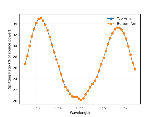
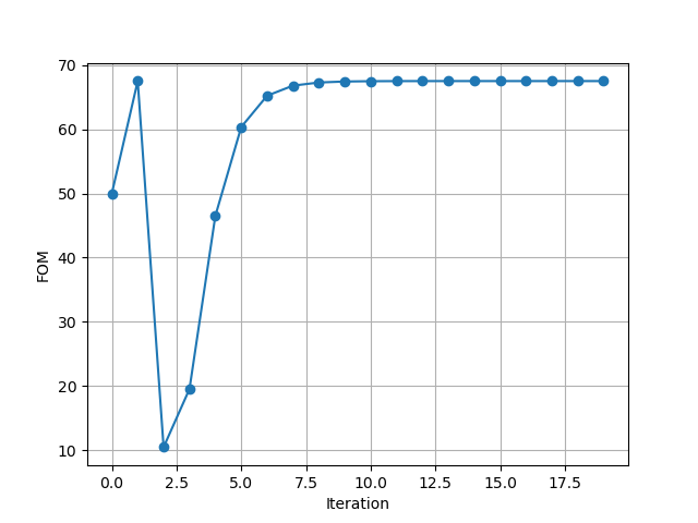
fcen=1/0.55andfwidth=0.3but limiting the wavelengths used in the objective function to [0.535, 0.575] I have better values for the initial monitor measurements and power splitting between the focus and antifocus region:However when I run this simulation for 20 iterations I get the following plot of how my figure of merit improves seems to taper off as can be seen in this plot:

The monitor measurements and ratios are:

So it does seem I get a little bit of an improvement in focusing onto the top source monitor, it is not uniform across spectrum and hardly improves after the 8th iteration
I have not (yet) incorporated any erosion or dilation filters. I assume these, while good for incorporating manufacturing constraints would hinder device performance, rather than boost it, and I want to find the source of the flattening of the FOM curve before complicating the problem further.
I would appreciate any advice on how to fix this or how to better understand what is going on so that I can be better equipped to solve these problems by myself in the future. am rather new to computational EM and am trying to develop a better understanding of setting up and modeling devices as well as debugging any issues with the simulations.
It would also be great to know is there a way to save and load OptimizationProblems? I assume its not the same as loading and dumping simulation state as that dumps epsion but OptimizationProblems take DesignRegions which store information about the ranges of epsilon
Additionally any advice for modeling the air-polymer device in the paper I posted would be tremendously appreciated.
The code for the simulation is:
Beta Was this translation helpful? Give feedback.
All reactions